This is the first of two writings talking about the difficulties of reasoning under uncertainty. Uncertainty is a fundamentally probabilistic concept; as such, our discussion might start with an examination of the foundations of probability itself. As with any concept as vague yet intuitive as probability, we ought to analyze it at multiple levels:
We'll start with the first point, surveying various different meanings of the word probability, before subdividing each meaning into a set of rigorous translations compatible with it; such a combination of a meaning and translation is known as an interpretation of probability. Finally, in order to cover the third point, we will draw out the implications of and paradoxes within each interpretation, as well as comparing their strengths and weaknesses relative to one another. It turns out that even something as intuitive as probability turns out to be an extremely thorny concept upon further examination, with every interpretation being either limited to an extremely narrow domain or prone to internal contradiction; in short, we'll discover why probability is difficult.
While I try to stay away from arguments via pure mathematics, seeking to translate them into conceptual terms, some parts are excessively technical. Some calculus, and a basic understanding of sets and set operations, is required to understand most of these.
Any introduction to probability will generally begin with a few classical examples — rolling die, flipping a coin, being dealt a certain hand from a deck, and so on. These intuition pumps allow us to examine the features of probability in the most basic cases. To introduce the main interpretations of probability we'll cover in this essay, let's go with a particularly contrived example of an uncertain die roll.
I videotape myself rolling a normal, six-sided die, and show this video to a small focus group of people, each of whom has a different idea of what probability means. As the die leaves my hand in the video, I pause it, and ask them what the probability that the die will land on an even number is.
Which justification do we take to be the most accurate? Obviously, the answer depends on what we mean by probability, but what exactly we mean can be very difficult to pin down. Many people have tried, coming up with many different answers, and we'll explore those in turn. Each of these "willing" participants has given a unique account: Carrie the Classical account, Barry the Bayesian account, Frank the Frequentist account, Paul the Propensity account.
💡 The major interpretations of probability theory are the classical, Bayesian (subjective), frequentist, and propensity interpretations.
There are some additional interpretations which I've neglected to list here: the Stanford Encyclopedia of Philosophy's article lists the evidential and best-system interpretations in addition to these four, but I found these to be relatively obscure. The latter piques my interest, though, and I may cover it in an addendum.
Before we go on to cover these interpretations, let's resolve one basic ambiguity resolving the use of the word probability. To introduce this ambiguity via metaphor: suppose that some alternate dialect of English did not have different words for what we call couches and beds, instead referring to couches, beds, and everything in between simply as bēds. Would we not then expect to see the speakers of that dialect arguing ferociously over whether bēds were for sitting or for lying down, whether blankets go on bēds, or how many people a bēd should be able to occupy? After all, all of those questions are a lot more ambiguous in their dialect than in ours!
The historical debate over probability is kind of like this, with the vocabulary provided to us by our language often being a major source of confusion. Just as it would be useful for the speakers of our strange dialect of bēd-English to distinguish between two different kinds of bēds — those that we call beds and those that we call couches — many authors on the subject of probability have suggested that it is necessary to distinguish between two separate uses of the word "probability".
💡 Colloquially, the word "probability" can refer to subjective levels of certainty, or to empirical frequencies; it is useful to disentangle these uses from one another.
Many of those noticing this distinction have gone on to give individual names to each of these independent uses. Unfortunately, they all seem to have come up with different names. Popper terms these uses "subjective" and "objective" probability, respectively; Hacking uses "epistemic" and "statistical", Gillies uses "logical" and "scientific". Carnap, never hesitant to express that legendary German creativity, uses "probability$_{1}$" and "probability$_2$". I prefer Popper's terminology, with the reasoning that subject-ive probability lies within the interpreting subject, while object-ive probability lies within the interpreted object.
Maher terms the second use "physical probability", and splits the first into "subjective probability", or the degree of belief held by an actual person, and "inductive probability", or the degree of belief that it is rational to hold. The notion of rationality is vague, but we'll see later that pretty loose interpretations of it can have pretty tight implications.
In terms of the interpretations we'll study below, the subjective sense of probability is taken implicitly by Bayesians, while the latter, objective sense is taken implicitly by frequentists; the classical and propensity interpretations often blur the line between the two.
The Bayesian-frequentist divide is one of the most significant in all of probability, but distinguishing between their uses of the word probability as being different uses of the word allows us to slightly defuse the debate: they are often not even speaking of the same thing. If I say “bēds are for sitting on” and you say “bēds are for sleeping on”, the debate may be defused by noting that I am referring to couches and you are referring to beds. Of course, this does not always work, and there are genuine conflicts between Bayesianism and frequentism, but this consideration demonstrates the great extent to which we can consider Bayesianism and frequentism as independent, rather than exclusive.
With that out of the way, let's cover each interpretation in turn.
This interpretation is intimately tied with the early development of the mathematical theory of probability itself, which was largely driven by French gamblers in the 17th and 18th centuries. In the 19th century, this interpretation was fully realized by the French non-gambler Laplace, who in his 1814 "A Philosophical Essay on Probabilities" writes:
The theory of chance consists in reducing all the events of the same kind to a certain number of cases equally possible, that is to say, to such as we may be equally undecided about in regard to their existence, and in determining the number of cases favorable to the event whose probability is sought. The ratio of this number to that of all the cases possible is the measure of this probability, which is thus simply a fraction whose numerator is the number of favorable cases and whose denominator is the number of all the cases possible.
The bolding is mine, and highlights the fundamental principles of the classical interpretation of probability: the probability of some event is the frequency of possible cases that give rise to that event in a collection of cases all of which are indistinguishable with respect to our information. If this number of total cases is $A$, and the number of cases which give rise to that particular event is $N$, then the probability of the event is simply $N/A$.
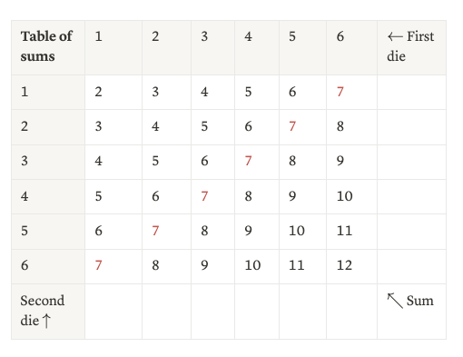
Example: Suppose we have two six-sided dice which we have no reason to believe aren't fair, and we would like to calculate the probability of a roll of these dice summing to seven. Since we have no reason to favor any combination of rolls over any other, the classical interpretation tells us to consider them all as being indistinguishable. So, the probability of a seven will be the number of combinations of rolls that sum up to seven divided by the total number of combinations of rolls. I've tabulated this below:
Hence, there are six combinations that yield a sum of seven, and thirty-six total combinations, giving us a probability of $6 / (6 \times 6) = 1/6$ of rolling a seven.
Let's now draw out the core mathematical and philosophical assumptions behind the classical interpretation of probability.
The first major distinction that we had to make in applying the classical interpretation to our toy example (rolling a seven) was as follows: on one hand, there are the events we sought to calculate probabilities of; on the other hand, there are the samples generating these events. In the sum of dice case, the events were “sum = n”, for n some given number. The samples generating these events, however, were individual combinations of die rolls. The set of all events for which we seek to calculate probabilities will be known as the event space, while the set of all samples will be known as the sample space.
Note: Clearly, we could've used the classical interpretation to calculate the probability of any given sample, i.e. combination, as being one in thirty-six, but in general we must specify our events, or the scenarios which we wish to calculate probabilities of, separately from our samples, or the underlying system configurations generating those scenarios. A horrific example of this will be given later, when we encounter Bertrand's Paradox.
Our notation going forward will be as follows: given a system, the set of all configurations of that system, or the sample space, will be denoted as $\Omega$, while the set of all collections of configurations whose probabilities we wish to measure, or the event space, will be denoted as $\mathcal F$. Each event, as mentioned, is really a collection of samples, i.e. a subset of $\Omega$.
Given that it's events whose probabilities we wish to measure, and that probabilities are numerical values, there must be a measure of probability $P: \mathcal F \to \mathbb R$ sending an event $F$ to its probability $P(F)$. This function $P$ is known as a probability measure. There are several implicit constraints on this probability measure embedded in the classical interpretation; let's pick them out.
The first implicit constraint is that the probability of any event must be between zero and one. To see this, simply re-read Laplace's expression: the probability of an event is the ratio of “the number of cases favorable to the event whose probability is sought” to “the number of all the cases possible”. Our more modern language replaces “case” with sample and “favorable” with “contained within”. Clearly, there cannot be a negative number of samples contained within an event, nor can there be more samples contained within an event than there are samples altogether, so the probability of an event must be between zero and one.
The second implicit constraint is that the probability of an event depends only on those samples making up the event. This follows from the above point. These two constraints yield a number of powerful rules.
It seems that the classical interpretation of probability actually yields a very detailed set of rules for calculating probabilities.
The distinguishing philosophical feature of the classical interpretation is its commitment to treating indistinguishable samples as equivalent. In other words, any two samples which we cannot distinguish between must be considered to contribute equally to the probabilities of all events of which they are members. This principle is known as the principle of indifference. This principle is ultimately what gave us the power to calculate the probability of rolling a seven as being one in six — without it, how could we reason about the contributions made by different combinations of die rolls (i.e., different samples)?
While the above rules for working with probabilities are commonly accepted nowadays, it is the principle of indifference which, as we'll see, ends up landing the classical interpretation in hot water.
💡 The classical interpretation is distinguished primarily by its reliance on the principle of indifference, which states that we should consider as having equal probability those possibilities which no information allows us to distinguish between. Implicit in it, though, is a set of rules for working with probabilities which continue to inform modern probability theory.
All of the examples we've given have dealt with finite sample spaces: the 36 possible combinations of two dice, the 2 possible results of one coin flip, and so on. It's not like enlightenment-era French gamblers ever worked with infinitely divisible roulette wheels or continuum-valued playing cards; whole numbers were all they needed to deal with, and all they designed the classical interpretation to be able to handle. Indeed, before Cantor's late 19th-century work, the notion of infinity itself was entirely unclear to mathematicians.
However, with the expansion of probability theory into other domains of reasoning, domains which involved continuous variables such as currency exchange rates or positions of particles, it rapidly had to learn to deal with sample spaces covering all possible values of these continuous variables, i.e. infinitely large sample spaces. This requires a subtle but fundamental shift in the language we use.
I'll walk us through this shift with a pedagogical example: suppose that we pick a random point on a circle, and want to ask ourselves about the angle of this point in degrees — how likely is it that it's between $90^{\circ}$ and $135^{\circ}$, or between $7^{\circ}$ and $(3\sqrt{10})^\circ$?
The point may take on any angle which is at least $0^{\circ}$ and below $360^{\circ}$, making the sample space $\Omega = [0, 360)$ — any angle in this range is a valid sample. What of the events, though? Whatever the events are, we must be able to calculate their probabilities according to the rules above.
Our first guess might be to make each sample its own event, such that for any position $x \in [0, 360)$ we can speak of the probability $P(\{x\})$ of the point being at precisely that position. However, since $\Omega$ is the union of all $\{x\}$, for $x \in \Omega$, the third rule sketched out previously would give us $$P(\Omega) = \sum_{x \in \Omega} P(\{x\}) = 1$$
Since there are uncountably many points in $\Omega$, this sum is particularly horrifying; its equality to 1 suggests that all but countably many points must have zero probability. (To prove this requires some mathematical subtlety, so take my word for it). As such, if we were to make every sample its own event, we'd inadvertently restrict the point to a vanishingly thin set of positions on the circle, rather than allowing it to be anywhere on the circle. This is clearly a bad idea.
Our second guess might be to make each interval between samples its own event, such that for any $a, b$ in$[0, 360)$ we can speak of the probability $P((a, b))$ of the point being between $a$ and $b$. This works out significantly better. (In almost all cases it does not matter whether we use $(a, b)$ or $[a, b]$; the former simply makes the math easier to work with).
The most common way to express these values is in terms of a probability distribution function (pdf) $p: \Omega \to \mathbb R$ such that $$P([a, b]) = \int_a^b p(x)\, dx$$ (This is often referred to as the probability density function. Both have the same acronym, thankfully).
Not all possible probability measures have pdfs, but almost all commonly-encountered ones do. (A sufficient condition for the existence of a pdf is that $P$ assign a probability of 0 to any event with length 0, a fact known as the Radon-Nikodym theorem). Therefore, when reasoning about continuous sample spaces $\Omega$, we shall assume that the probability function $P$ from the event space $\Omega$ to $[0, 1]$ arises from a pdf: $$P(F) = \int_F\, p(x)\, dx$$
In other words, the probability of an event is given by the integral over that event, when considered as a subset of the sample space $\Omega$, of the probability distribution function $p: \Omega \to \mathbb R$. This pdf must be normalized, in the sense that its integral over the entirety of $\Omega$ is equal to 1: $\int_\Omega p(x)\, dx = P(\Omega) = 1$.
Note that this formula for calculating the probabilities of events doesn't depend on the actual structure of the event space: the event space may be generated by intervals, or it may be of some other form. There are some coherence conditions that must be placed on the structure of the event space and the pdf in order for this integral to always be well-defined, but these arise within the framework of measure theory and Lebesgue integration, which is far too complex for us to cover here.
Let's stick with the circle example, with sample space $\Omega = [0, 360)$, events being given by intervals $(a, b)$, and probabilities of events being derived from some pdf $p$ as $P((a, b)) = \int_a^b p(x)\, dx$.
How do we express the principle of indifference in this new, continuous framework? The first step is to note that any sample $x$ contributes to a probability $P((a, b))$ only through the value of $p(x)$. The principle of indifference asks us to ensure that any two samples which we can't distinguish between make the same contributions to all probabilities which they're a part of, and we certainly have no reason to distinguish between two different points on the circle — it's rotationally symmetric!
As such, the only pdf consistent with the principle of indifference is the pdf that assigns the same value to each point. In other words, $p(x) = c$, where $c$ is some constant, for all $x \in \Omega$. We may find this constant by noting that $P(\Omega)$ must be equal to $1$: $$1 = P(\Omega) = \int_\Omega p(x)\, dx = \int_0^{360} c\, dx = 360c \implies c = \frac1{360}$$
Therefore, the principle of indifference gives us a unique pdf on the circle, and therefore a unique probability for each event $F = (a, b)$: $$P(F) = \int_F p(x)\, dx = \int_a^b \frac{1}{360}\, dx = \frac{b-a}{360}$$
In other words, the probability of an event under this distribution is determined entirely by the proportion of the sample space it spans. As such, this $P$ is known as a uniform measure; its pdf is known as a uniform distribution.
In general, the principle of indifference guides us to use a uniform measure, both on infinite sample spaces and on finite ones — in both cases, this measure sets $P(F)$ equal to the proportion of the sample space taken up by $F$, whether this be the length of $F$ divided by the length of the (infinite) sample space, or the cardinality of $F$ divided by the cardinality of the (finite) sample space.
Sometimes we may be able to construct multiple sample spaces corresponding to the same system, with each space capturing all the information we need. Wiki has a very nice example, which I'll remix: Suppose you buy a tungsten cube so your friends think you're cool, but don't know its mass: all you know is that it could be anywhere between 3 and 3.1 inches on a side. The density of tungsten is known, so all you need to do is estimate its volume. There are two ways to use the principle of indifference to do this:
These are different answers! To show exactly why this is the case, we have to discuss the reparametrization of probability distributions in general.
Suppose we have two different sample spaces $\Omega_1,\Omega_2$ which we can use to model a system, and an invertible function $f: \Omega_1 \to \Omega_2$ expressing the fact that they capture the same information. If we have a probability measure or pdf on $\Omega_1$, we may define a probability measure on $\Omega_2$ by letting the measure of some interval $[a, b]$ in $\Omega_2$ be the measure of the interval $[f^{-1}(a), f^{-1}(b)]$ in $\Omega_1$. This is known as the change of variables of $p_1$ by $f$. For instance, in the above example, we have $\Omega_1 = [3, 3.1]$ as the side length sample space, while $\Omega_2 = [27, 29.791]$ as the volume sample space.
If we have a pdf $p_1$ on $\Omega_1$ corresponding to a probability function $P_1$, then we may calculate probabilities on $\Omega_2$ by using $f$ to obtain a second pdf $p_2$ as the pdf of the probability function $P_2([a, b]) = P_1([f^{-1}(a), f^{-1}(b)])$. By the fundamental theorem of calculus, $$p_2(v_0) = \lim_{h \to 0} \frac{1}{h} P_2([v_0, v_0+h]) $$ Plugging in the definition of $P_2$, we get $$\lim_{h \to 0} \frac{1}{h} P_2([v_0, v_0+h]) = \lim_{h \to 0}\frac1h P_1([f^{-1}(v_0), f^{-1}(v_0+h)]) \\ = \lim_{h \to 0} \frac1h P_1([f^{-1}(v_0), f^{-1}(v_0) + \frac{df^{-1}(v_0)}{dv}h + O(h^2)]) \\ = \left|\frac{df^{-1}(v_0)}{dv}\right|p_1(f^{-1}(v_0))$$ the absolute value symbol coming from the fact that the limit is independent of the direction of the derivative, only its magnitude: if $b > a$, then $[b, a]$ and $[a, b]$ are the same interval; all flipping the direction does is cause us to take the limit from the left rather than from the right, but if $f^{-1}$ is to be differentiable at $v_0$ at all, the limit must be the same from the left or right. For instance, when $p_1$ is the uniform distribution on side lengths, $p_1(\ell) = \frac{1}{3.1-3} = 10$, and $f$ sends a side length $\ell$ to its volume $v = \ell^3$, then $p_2(v) = \frac{10}{3\sqrt[3]{v^2}}$, which is not uniform: $p_2(3^3) = \frac{10}{27}$, while $p_2(3.1^3) = \frac{10}{28.83}$. However, if we calculate the probability of the mass being below 300 oz using this distribution on the volume, we get the same answer as we did with side lengths, 10.07%.
Changing a uniform distribution via a function $f$ only results in another uniform distribution when the derivative of $f$ is constant — in other words, when it scales samples from the first space into samples from the second space. In our case, $f$ cubes a side length to get a volume, and therefore does not yield a uniform distribution. Hence, when we used a uniform distribution for the volume, we were in reality using an entirely different distribution than the one we would have derived from the side length. Why, then, should we get the same answer?
The fact that changing of variables almost never preserves the uniformness of a distribution means that the principle of indifference forces us to choose a specific parametrization of a problem before we can use it, and this choice matters — choosing any two different parametrizations that aren't just multiples of one another will give us different probability distributions!
The most famous example of this is Bertrand's paradox.
A question: What is the probability that a chord which is not a diameter, randomly selected from within a circle of radius $2R$, intersects the concentric circle with radius $R$?
(I've taken this particular formulation from Evans' SDE book, with regularization to remove the problem of diameters as per source. The usual formulation asks whether the chord is shorter than any side of an equilateral triangle which the circle circumscribes, but these two formulations are essentially equivalent).
Why is this a paradox? We can use the principle of indifference in three different ways to get three different answers.
Each of the three different methods of picking chords corresponds to a different probability distribution over the chord space $\mathcal C$; if we let $I$ be the set of all chords that intersect the inner circle and $O = {\mathcal C} - I$ the set of chords that don't, the answer given by a probability distribution $p$ over $\mathcal C$ will be given by $\int_O p\, dO = 1 - \int_I p\, dI$, $\int_O p\, dx = 1 - \int_I p\, dI$.
1. When we identify $\mathcal C$ with the circle itself (sans center and edge) by sending a chord to its midpoint, the first method obviously corresponds to a uniform distribution. $p = \frac{1}{4\pi R^2}$. $I$ is identified with the inner circle and $O$ with the outer annulus (ring), so $\int_I p\, dI$ is just the area of the inner circle, or $\pi R^2$, divided by $4\pi R^2$; this gives us the $1/4$ answer we arrived at previously.
2. The set of all chords that can result in a vertical chord $c$ away from the center is identified with the set of all points of the circle that are themselves $c$ away from the center; the measure of this circle $S_c$ under the uniform distribution is $\int_{S_c} p\, dS_c = 2\pi c/4\pi R^2 = c/2R^2$, but under the distribution $p'$ corresponding to this method, the measure of $S_c$ must be a constant $k$, independent of $c$, since we're choosing vertical chords uniformly; we have $$1 = \int_{\mathcal C} p'\, d{\mathcal C} = \int_0^{2R} \int_0^{2\pi} r p'(r, \theta)\, d\theta\, dr = \int^{2R}_0 \left(\int_{S_r} p'\, dS_r\right)\, dr = \int_0^{2R} k \, dr = 2kR$$ and therefore $k = 1/2R$. It follows that $$\int_I p'\, dI = \int_0^R \int_0^{2\pi} rp'(r, \theta)\, d\theta\, dr = \int_0^R \frac{1}{2R}\, dr = \frac{R}{2R} = \frac12$$ so that this method of choosing chords randomly gives a different probability distribution which integrates across $I$ to give $1/2$.
3. This one is significantly trickier to set up the measure for. If we take the x-axis of a point chosen on the upper edge of the circle, we're significantly more likely to get a value closer to $\pm R$ than to $0$ due to the sides becoming vertical at $\pm R$ and therefore contributing significantly more mass; this privileges chords that are very close to being tangents and chords that are very close to being diameters. I think that the distribution is $\displaystyle p''(r, \theta) = \frac{2}{(2\pi r)^2\sqrt{\frac{4R}{r} -1}}$, so that $$\int_I p''\, dI = \int_0^R\int_0^{2\pi} \frac{2r}{(2\pi r)^2\sqrt{\frac{4R}{r}-1}} \, d\theta\, dr= \int_0^R \frac{1}{\pi\sqrt{r(4R-r)}}\, dr \overset{m=r/2}= \int_0^{R/2} \frac{1}{\pi\sqrt{m(2R-m)}}\,dm=\int_0^{R/2} \frac{1}{2\pi R\sqrt{\frac{m}{2R} - \frac{m^2}{4R^2}}}\, dm \overset{u=m/2R}{=} \int_0^{1/4} \frac{1}{\pi\sqrt{u-u^2}}\, du = \frac13$$ (calculation) but I'm not sure how to convincingly justify it.
Hence, Bertrand's paradox lies in the word "random": we're choosing a chord from one of the three different midpoint distributions $$p(r, \theta) = \frac{1}{4\pi R^2} \quad p'(r, \theta) = \frac{1}{4\pi rR} \quad p''(r, \theta) = \frac{2}{(2\pi r)^2\sqrt{\frac{4R}{r}-1}}$$
Someone trying to solve this problem would likely just pick the first of these methods that appealed to them, calculate the corresponding probability, and conclude that they have “the” answer. We see that the principle of indifference can, if used unscrupulously, mislead us. It has been asserted, most famously by E. T. Jaynes (here), that by extending the principle of indifference to the notion that the solution should be invariant under translation, rotation, and scaling of the circle, we get a unique solution ($1/4$), and he claims to have experimentally demonstrated this by throwing straws at a circle drawn upon the ground (thereby also experimentally demonstrating all the hubris of a Bayesian and a physicist!). It has been argued in return (e.g. here) that "The straw throwing experiment is not the empirical confirmation of an independent abstract analysis. Instead, the analysis is a mathematization of the straw throwing procedure", and that a similar analysis can give the other two answers as well.
💡 Bertrand's paradox demonstrates that the principle of indifference often fails to give clear answers when the underlying sample space is continuous, rather than discrete.
Earlier, we used the principle of indifference to find a suitable probability distribution for a point randomly selected from a circle. This worked because the sample space — the circle itself, or equivalently the set of angles on the circle — was compact: the integral of a constant function over it converged to a single number, the reciprocal of which formed our constant pdf. This is often not the case, though, and in such cases the principle of indifference drives us straight into a wall.
For instance, consider the problem of picking a random real number, when no information is available to guide our choice. The principle of indifference suggests that we do this according to a uniform distribution on $\mathbb R = (-\infty, \infty)$, but there can be no such distribution: if the distribution is given by $p(x) = c$, then we must have $1 = P(\mathbb R) = \int_{-\infty}^\infty p(x)\, dx = c\times \infty$, which makes no sense.
Jaynes, again, attempts to solve this. This time, he provides us with the principle of maximum entropy: given a sample space $\Omega$, we should pick the probability measure $P$ with pdf $p$ such that the entropy $$H[p] = -\int_{\Omega} p(x) \ln p(x)\, dx$$ is maximized. (The notation $[-]$ is sometimes used to denote functionals, or functions of functions). Entropy is generally taken to be the absence of built-in information, so maximizing entropy minimizes information. Indeed, when $\Omega = [a, b]$, such that we can construct a uniform distribution on it, then the maximum entropy probability distribution is that uniform distribution.
There is no maximum entropy probability distribution on $(-\infty, \infty)$ — we can construct a distribution with arbitrarily high entropy — though one becomes available if we are willing to specify some additional information about the distribution. Most famously, the maximum entropy probability distribution with a specified mean and variance is the normal distribution (aka bell curve, Gaussian distribution) with that mean and variance. Hence, in itself, the principle of maximum entropy is not a solution to the problem of non-normalizability, merely a heuristic.
Hence, while the classical interpretation of probability gives us a reasonable way to solve probability problems involving finite sample spaces, it fails dramatically in infinite spaces due both to ambiguities it fails to resolve (and tricks us into thinking we have resolved!) as well as the fundamental impossibility of constructing uniform distributions over unbounded spaces such as $\mathbb R$.
💡 We can't even construct uniform distributions over many spaces which we'd like to consider probability distributions on, further hampering the principle of indifference.
(There have been some silly attempts to yield a canonical answer to Bertrand's paradox by blending together various probability distributions on the chord space $\mathcal C$ in order to get a "canonical" one, which supposedly would give the right weighting and therefore the right answer. Shackel develops a principle of metaindifference, in which we apply the principle of indifference to the probability distribution on $\mathcal C$ themselves, taking them to be equally probable and therefore averaging them out to get a canonical solution; he quickly admits that this doesn't work for the obvious reason — there are uncountably many measures, so we need a measure on the measure space to average them out, but which one? We get an infinite regress).
Just to rub it in, we'll give an example where the principle of indifference produces ambiguities in the finite setting. Originally expressed in this form by Shafer in his “A Mathematical Theory of Evidence”, this example goes as follows: Suppose we're trying to reason about the existence of life on some planet orbiting the star Sirius, without incorporating any prior information about the plausibility of aliens or Sirius itself.
We might say that there are two possibilities: either there is or there isn't, and use the principle of indifference to apply a probability of 1/2 to both. On the other hand, we might say that there are three possibilities: either there is a planet containing life, none of its planets contain life, or there are no planets around Sirius. Applying the principle of indifference here has us assign a probability of 1/3 to the presence of life, rather than 1/2. Even in the finite case, the principle of indifference can yield different answers based on how we formulate the problem.
Some definitions, to formalize the situations we've already been dealing with:
We've already introduced event spaces $\mathcal F$ as being collections of subsets of some sample space $\Omega$, and have demonstrated that they are closed under unions, intersections, and complements, and contain $\emptyset$ and $\Omega$.
The functions we've placed on $\mathcal F$ have generally been non-negative functions which send $\emptyset$ to 0. I
One famous method of summing up these properties of a probability measure is via the three axioms:
These are known as the Kolmogorov axioms, and form the basis for most axiomatic treatments of probability theory. Sometimes, though, additivity is only taken to hold for finite, rather than countable, collections of events; this doesn't change much practically, but breaks a lot of measure-theoretic proofs which require countable additivity. The notion of a probability space underlies almost all of the classical probability that we will be talking about.
💡 Formally speaking, a probability space is a measurable space equipped with a measure which is unitary, non-negative, and countably additive (Kolmogorov's axioms).
Kolmogorov's axioms are incredibly useful in part because they are interpretation-agnostic: use of them does not commit us to any particular interpretation, and we shall see that it makes sense to adopt them in many different interpretations of probability; in all of these, they form a useful base from which to understand the notion of probability advocated by that interpretation.
This interpretation-agnosticism is to be contrasted with operationalist foundations, which define probability by operationalizing it, i.e. by putting it in terms of observable entities rather than as some symbol satisfying some properties. As we'll see, this operationalist foundation, initially developed by Richard von Mises, often commits us to a frequentist interpretation, though frequentism may extend past it.
To a Bayesian, also known as a subjective probabilist, a probability is a degree of belief. Actual observation is not necessary to generate probabilities, as it is to frequentists, but it is the ultimate test of such partially-held beliefs — if they are rational, you should be able to use these beliefs to bet on what observations you will make, and end up making money.
As mentioned above, Bayesians disagree over whether any partial beliefs are probabilities, or rational partial beliefs are probabilities. Again, terminology abounds: some call the latter belief inductive probability, others logical probability.
For instance, if I subjectively place a probability $p > 0$ on some particular horse H winning a race, and you place a probability $1 > q > p$ on H winning, we should (if we both really believed in those probabilities, and had money to spare) agree on the following bet:
No matter what the actual probability of H winning is, clearly one of us must be wrong to accepting this bet — since money doesn't appear from thin air, it would be impossible for the to actually benefit both of us. The person whose probability is more accurate will end up gaining, on average, from this bet. Thus, subjective probabilities can be tested.
💡 Bayesian probabilities are degrees of belief; insofar as they are taken to be rational, they can be decisively tested by seeing whether actions taken on these beliefs, such as the taking or rejecting of bets, are rational.
A perfect Bayesian reasoner should be able to set their probabilities such that they never make a bet with negative expected value. Careful analysis of this statement shows that the inferences of such a reasoner must follow a particular logic. This logic is traditionally derived via the "Dutch book" argument, which constructs a series of bets (a Dutch book) that a reasoner is guaranteed to lose money on if their probabilities do not follow a set of rules. These rules, and the corresponding books, are:
These are the Kolmogorov axioms, albeit with only finite additivity. It can be shown that they are not just necessary, but sufficient, for a Bayesian reasoner to be able to avoid all Dutch books (one proof is here).
💡 The analysis of Dutch books shows that rational subjective beliefs must necessarily follow the Kolmogorov axioms.
Because ideal Bayesian reasoning satisfies (a slightly weakened version of) Kolmogorov's axioms, Bayesians implicitly use the same framework as classicists, working in a measure space $(\Omega, {\mathcal F}, P)$. However, because their framework of subjective probability strongly emphasizes updating on observations, they're keen on switching between spaces. If an event $A$ is observed, for instance, why not restrict the entirety of the measure space to $A$? In this case, we can let the probability measure $P_A$ of the new space be given by $P_A(B) = \frac{P(B \cap A)}{P(A)}$; dividing by $P(A)$ guarantees unitarity of $P_A$, and intersecting $B$ with $A$ takes only that part of $B$ that is known to concord with $A$ (as, having observed $A$, the rest must not be the case). This process is known as conditionalization, and we generally write the quotient $\frac{P(B\cap A)}{P(A)}$ as $P(B \mid A)$, where $B \mid A$ is read as "B given A"; this probability can be interpreted as the probability of $B$, given that we know $A$ to be true.
Clearly, $P(B \mid A) P(A) = P(B \cap A)P(A)=P(A \cap B) = P(A \mid B)P(B)$. Dividing both sides by $P(B)$ gives us Bayes' theorem, $$P(A \mid B) = \frac{P(B \mid A)P(A)}{P(B)}$$
In the context of conditioning upon observation of some event $B$, $P(A)$ is called the prior probability of $A$, while $P(A \mid B)$ is called the posterior probability.
💡 Observation of a particular event allows us to restrict our measure space to the measure subspace on that particular event, with the natural alteration to the probability measure being encoded by Bayes' law.
One controversial aspect of Bayesian reasoning is its tendency to assign subjective probabilities to anything that isn't known to the reasoner, such as the current position of Mars or the number of beans in a jar; we might give the former a uniform distribution along the orbit, and the latter a normal distribution centered around a Fermi estimate (or a wild guess). The origin of priors is one of the largest issues with Bayesian reasoning. There are two major families of answers to the question "whence priors?":
Hence, the question of where priors come from, when it is answered at all, only serves to open up Bayesianism to the same counterarguments as were provided against the classical interpretation: for one, the ambiguity of the principle of indifference and lack of applicability of the maxentropy principle. Furthermore, the question of constructing priors is just as susceptible to the reference class problem explored in the propensity interpretation.
💡 Bayesianism's greatest vulnerability lies in the origin of prior probabilities. If these are to be arbitrary, they can be nonsensical; if they are to be rational, they can still be ambiguous and misleading.
A common heuristic for judging priors is complexity: the idea is that we should, ceteris paribus, choose those priors that are as simple as possible. This drives the maxentropy principle, which takes complexity to be low entropy, as well as the more common reasoning principle known as Occam's razor.
The most powerful complexity-penalizing rule for building priors is Solomonoff's algorithmic probability. The main drawback of the algorithmic probability framework is that it's very formal, and inapplicable to most real-world problems, but it's still very morally interesting.
Fix a universal Turing machine $U$ with alphabet (symbol space) $\{0, 1\}$. This UTM will compute anything that can be computed, and in particular a pre-selected finite bit-string $X$, so long as it's given the right program ${\tt p}$. We do not consider the UTM as being fed a program and then information; the information is taken to be part of that program. Writing $\{0, 1\}^*$ for the set of all finite bit-strings, we can therefore consider $U$ to be a map $\{0, 1\}^* \to \{0, 1\}^*$, where elements of the domain are treated as input programs and elements of the range are treated as output data. $U^{-1}(X)$, then, is the set of all programs ${\tt p}$ which produce $X$ when fed to $U$.
There may be multiple programs $\tt p$ such that $U({\tt p})$, the result of feeding $\tt p$ to our fixed UTM, yields $X$ (i.e., $U^{-1}(X)$ may have more than one element), and we define the Kolmogorov complexity of $X$ to be $$K(X) = \min_{{\tt p} \in U^{-1}(X)} \ell({\tt p})$$
Here, $\ell(\tt p)$ is the length of the program $\tt p$, which is a measure of its complexity. The Solomonoff prior $P_S$ is given by $$P_S(X) = \sum_{{\tt p} \in U^{-1}(X)} 2^{-\ell({\tt p})}$$
The weight $2^{-\ell({\tt p})}$ is the probability that a randomly chosen bit-string of length $\ell({\tt p})$ will be ${\tt p}$ itself. Thus are more complex (i.e. longer) programs penalized.
There will always be some program that produces $X$ — say, the program that says "print the following data and then halt: $X$", so that $P_S(X)$ will never be zero. In fact, $P_S(X)$ will always be at least $2^{-K(X)}$, since the $X$-producing program with minimal length will be included in this sum.
Provided we limit our choice of $U$ to a certain class of "prefix" UTMs, $P_S$ is well-defined; remarkably, the choice of $U$ only affects priors up to a constant.
Drawbacks:
Thus, there are all sorts of schemes for approximating Solomonoff's universal prior, as well as for including things in it like penalties for using excess time or space. (An anthropic viewpoint might say, for instance, that the very fact that we're seeing such-and-such data should bias us towards thinking it was generated by processes that produced it quickly, as otherwise we wouldn't've noticed it, or it wouldn't have finished computing in the measly 1.4e10 years the universe has existed for).
💡 Solomonoff's universal prior is a way to weigh the prior likelihood of data based on the necessary complexity of its generating processes, though it's far from practical.
David Lewis' Principal Principle is a possible restriction one might make on subjective probabilities. Consider a proposition $\Omega$ stating that the probability of some other proposition $X$ at time $t$ is $x_0$. The PP says that if $P$ is the subjective probability function of a reasoner, then $P(X \mid \Omega, Y) = x_0$ for any $Y$ which is admissible for $X$ at time $t$. By “admissible at a time”, we mean that $Y$ does not contain any information that overrides $\Omega$ at that time. If for instance it logically entails $X$ at some point in the future, then $P(X \mid \Omega, Y)$ should unequivocally equal another probability at that future time.
In other words, the PP says that subjective probability should concord with propositions about physical probability, or chance — if we know the chance of something, then we should generally set our subjective probability equal to that chance.
It has been shown that, under some conditions, PP implies a weak version of PI, namely the statement that binary propositions for which we have no information should rationally be given probability 1/2. Note that this excludes propositions like “my face is made of butter”, which we have extremely low credence in as a result of our background knowledge of what faces are made of and what things tend to be made out of butter, as well as “you will die on a Tuesday”, since we have the background knowledge that Tuesday is but one of seven days.
The argument given in the paper The Principal Principle Implies the Principle of Indifference is as follows: Let $F$ be a proposition which does not itself inform us about its own probability (e.g., it is neither a contradiction nor a tautology), and which we have no background information about. Let $\Omega, X$ be $F$-independent propositions such that $P(X \mid \Omega) = x_0 \in (0, 1)$, for instance as above. Let $Y$ be another $F$-independent proposition admissible wrt $\Omega$ at some time $t$, and let $(F \Leftrightarrow X)$ be the proposition “$F$ iff $X$”. By independence, $P(X \mid F, \Omega, Y) = P(X \mid \Omega, Y) = x_0$. We also have $P(X \mid (F \Leftrightarrow X), \Omega, Y) = P(X \mid F, \Omega, Y) = x_0$, as in the LHS $X$ obtains iff $F$ does, so the probability is unchanged by conditioning on $F$ rather than $(F \Leftrightarrow X)$. By Bayes' theorem, then, $$\frac{P(F \mid X, \Omega, Y) P(X \mid \Omega, Y)}{P(F \mid \Omega, Y)} = P(X \mid F, \Omega, Y) = P(X \mid (F \Leftrightarrow X), \Omega, Y) = \frac{P((F \Leftrightarrow X) \mid X, \Omega, Y)P(X \mid \Omega, Y)}{P((F \Leftrightarrow X) \mid \Omega, Y)} $$ The numerators of both fractions are equal, and both sides are equal to $x_0$, so the denominators are equal as well; that is, $P(F \mid \Omega, Y) = P((F \Leftrightarrow X) \mid \Omega, Y)$. However, we can infer that $P((F \Leftrightarrow X) \mid \Omega, Y) = P(\neg F, \neg X \mid \Omega, Y) + P(F, X \mid \Omega, Y)$, which can be written as $$P(F, X \mid \Omega, Y) + P(\neg F, \neg X \mid \Omega, Y) = P(F \mid X, \Omega, Y)P(X \mid \Omega, Y) + (1-P(F \mid \neg X, \Omega, Y))P(\neg X \mid \Omega, Y) = x_0P(F \mid \Omega, Y) + (1-x_0)-P(F \mid \Omega, Y)(1-x_0)$$ It follows that $P(F \mid \Omega, Y) = x_0P(F \mid \Omega, Y) + (1-x_0) - P(F \mid \Omega, Y)(1-x_0)$, which gives us $P(F \mid \Omega, Y) = \frac12$. Since $\Omega, Y$ are unrelated to $F$, we must have $P(F) = \frac12$ at this time as well.
In the propensity interpretation, probabilities are located in the physical world — it is the tendency of some system to result in some state some proportion of the time.
In either case, though, the propensity of the system to output a certain result is considered as a result of the preconditions, or environment, and of the system itself.
💡 To interpret probabilities as the propensities of systems to result in certain outcomes, whether on any particular trial or over an aggregate of many trials, is to place probabilities in the physical world.
Single-case propensity interpretations were first created by Karl Popper with the intent of making sense of quantum experiments: if $|\phi\rangle$ and $|\psi\rangle$ are two orthonormal eigenkets of some operator which is to be observed, and we have a particle in a superposition $\frac{\sqrt 2}{2}|\phi\rangle + \frac{\sqrt 2}{2}|\psi\rangle$, observation will cause the wave function of the particle to collapse into either $|\phi\rangle$ or $|\psi\rangle$, each with probability $\frac12$ — and this is the probability even if we only have a single particle in a single experiment. Neither the Bayesian nor frequentist interpretations seem to be able to say what this probability means, even though they're both capable of working with it. To be sure, there are interpretations of quantum mechanics that entirely avoid probability, but we can't take them for granted.
However, if we are to consider the propensity of some more mundane single case — say, the propensity of this coin I'm holding to land on heads – we quickly run into a complication:
And so on: all of these change the propensity slightly, and we can only speak of it as being 1/2 in the purely abstract case, even though the propensity derives from the generating conditions themselves! If we include every property of the coin flip which can affect its probability, though, we end up with a description so detailed that the coin flip is purely deterministic, so that its propensity is entirely to land on this side at this point on the table after this series of tumbles and so on. We must necessarily omit some detail if we're to have an actual probability, though which detail?
This problem — of finding out just how much detail to include — is known as the reference class problem. (See Gillies (2000), which uses the example of the probability of a 40 year old Englishman dying before 41).
One proposed solution is to simply say that single-case probabilities are subjective, being at best based on objective probabilities. At this point, the propensity interpretation rapidly gives way to a blend of frequentism and Bayesianism — we ought to pick the narrowest reference class for which we have statistical data, taking this data into account to refine our subjective probability. There is nothing new here.
💡 Single-case propensities, originally developed to deal with quantum mechanics, are difficult to consistently apply in other situations without arbitrarily picking some reference class or falling into Bayesianism.
It is clear from the above discussion that single-case propensity generalizes and critically depends on causality: to say that a system has a propensity $p$ of generating a given outcome is to say that it causes that outcome a proportion $p$ of the time. Suppose we have a system $S$ which has outcome $A$ with propensity $P(A)$, and which later has outcome $B$ with propensity $P(B)$, which outcome can be affected by $A$. We can then interpret $P(B \mid A)$ as the propensity of the system, given that it has caused $A$, to go on and cause $B$. How, then, are we to interpret the probability $P(A \mid B)$, which we can clearly calculate as $\frac{P(B\mid A)P(A)}{P(B)}$? It's accepted that effects come after causes, so $B$ cannot in any way cause $A$.
To paraphrase Gillies quoting an example from Salmon, if $A$ is my shooting some unfortunate person in the head and $B$ is that person dying, it's pretty clear how to interpret $P(A)$, $P(B)$, and $P(B \mid A)$. Suppose that these numbers are such that we calculate $P(A \mid B)$ as 3/4; would we then say that "this corpse has a propensity of 3/4 to have had its skull perforated by a bullet"? This seemingly nonsensical interpretation of retrocausal conditional probabilities is known as Humphreys' paradox, after Paul Humphreys, who described it here.
There are four proposed solutions:
Suppose a photon is shot in the vague direction of a half-silvered mirror, and call the event of its hitting the mirror $I$. Call the event of it passing through the mirror $T$. Since the mirror is half-silvered, the photon may not pass through — there's a non-zero propensity, or probability, $P(T \mid I)$, for it to pass through. Since the photon was not shot directly at the mirror, it may not even touch the mirror — there's a $P(I) \in (0, 1)$. If the photon never hits the mirror, though, it cannot pass through the mirror: $P(T \mid \neg I) = 0$.
By Bayes' theorem, which follows from Kolmogorov's axioms, we have $$P(I \mid T) = \frac{P(T \mid I)P(I)}{P(T \mid I)P(I) + P(T \mid \neg I)P(\neg I)} = \frac{P(T \mid I)P(I)}{P(T \mid I)P(I)} = 1$$
which makes sense from a common-sense Bayesian standpoint — if the photon passed through the mirror, then it definitely had to hit the mirror. This immediately contradicts CI, ZI, and NP, and since Bayes gives $P(I \mid T) = 1$ regardless of whether $I$ happened or not, it contradicts F as well. So, no matter what resolution to Humphreys' paradox we choose, if we're to stick with single-case propensity, we have to ditch Kolmogorov's axioms.
💡 To call a probability a propensity is to make it a causal phenomenon, which makes inverse conditional probabilities incoherent. This situation (Humphreys' paradox) cannot be resolved without ditching Kolmogorov's axioms.
Some people especially dedicated to single-case propensity have taken this as a cue to seek different axiomatizations of probability. One of these is Rényi's system, expounded in his 1955 paper On a New Axiomatic Theory of Probability.
This takes a measurable space $(S, \mathcal A)$ and adds to it a set of specified events ${\mathcal B} \subset \mathcal A$, the only restriction of which is that $\emptyset \notin \mathcal B$. There is a function $P: {\mathcal A} \times {\mathcal B} \to \mathbb R$, denoted $P(A \mid B)$, satisfying the following criteria:
If these are satisfied, then the tuple $(S, {\mathcal A}, {\mathcal B}, P)$ is known as a conditional probability space.
Every Kolmogorov (normal) probability space $(S, {\mathcal A}, P)$ generates a conditional probability space if we take $\mathcal B$ to be the set of events with non-zero probability and define $P(A \mid B)$ in the usual way, i.e. $P(A \cap B)/P(B)$, and conversely, every conditional probability space $(S, {\mathcal A, B}, P)$ generates a Kolmogorov probability space $(S, {\mathcal A}, P(- \mid B))$ for every fixed $B \in \mathcal B$.
Hence, conditional and Kolmogorov probability spaces are tightly connected, the main difference being that conditional probability spaces only allow us to condition on a certain pre-defined set of events, rather than all events.
So, to resolve Humphreys' paradox, we can simply say that we can condition on $I$ in the above example, but not $T$, so that $P(I \mid T)$ is simply undefined — we take option NP. This makes adoption of the Rényi axioms a partial solution for true believers in the single-case propensity interpretation.
It is a short-lived solution, however, since if in our conditional probability space something can be conditioned on $T$, then anything can be conditioned on $T$. To use the example in this paper, if we take two different fair die that are causally separated from one another, for instance by virtue of being in entirely different light cones, let $B, B'$ be the condition that each of them is rolled, and let $A, A'$ the condition that they land on one, then clearly $P(A \mid B) = P(A' \mid B') = 1/6$. But, if we admit that we can condition on $B$ and $B'$, then we must admit that we can define the cross-conditions $P(A \mid B'), P(A' \mid B)$, contradicting our choice of NP as a resolution to Humphreys' paradox. This is known as Sober's problem.
Instead of letting $P(- \mid -)$ be a function from $\mathcal A$ times a subset of $\mathcal A$ into $\mathbb R$, it might be better to write $P(- \mid -): \coprod_{A \in \mathcal A} {\mathcal B}_A \to \mathbb R$, where each dependent type ${\mathcal B}_A$ is a subset of ${\mathcal A}$ consisting of all those events which can have some causal effect on the event $A$. (Then, we'd hope for some criterion by which we can define each ${\mathcal B}_A$ in a nice manner, such as "the set of all events with $A$ in their future light cone, or in the same point in spacetime").
I don't know if this has been done; it would be tricky to find the right adaptation of Rényi's third axiom to the interplay of fibers ${\mathcal B}_A$ and inverse fibers ${\mathcal A}_B = \{A \in {\mathcal A} \mid B \in {\mathcal B}_A\}$ present in these "dependent" conditional probability spaces.
💡 Rényi's conditional probability spaces are weaker than Kolmogorov probability spaces; though they alleviate Humphreys' paradox, they quickly fall prey to the similar Sober problem.
Here, we consider the probability of some event to be the limiting frequency of that event as produced by a set of repeatable conditions, calling that probability a propensity of those conditions to result in that event. Gillies denotes this set ${\bf S}$, its set of possible outcomes $\Omega$, and defines events to be subsets of $\Omega$ (thankfully, agreeing with the measure theoretic framework). Hence, in this interpretation we can only speak of the probability of some event $A$ if we take it to be an outcome of some set of repeatable conditions $\bf S$; we must implicitly condition on it. The conditional probability $P(A \mid B)$, then, is to be interpreted as follows: take an ensemble of repetitions of $\bf S$, discarding all repetitions where $B$ did not happen, and take the limiting frequency of $A$ in this filtered set of repetitions. Clearly, this sidesteps Humphreys' paradox, but it does so by cruelly denying a causal interpretation of conditional probabilities.
💡 The long-run propensity interpretation is hipster frequentism.
In an experiment, the frequency of some event is the quotient of the number $m$ of occurrences of that event by the number $n$ of runs of that trial. For the frequentist, this frequency is the probability. The major distinction is whether this frequency is taken after some finite number of trials, a position known as finite frequentism, or whether it is taken to be the limiting frequency after an infinite number of trials, a position known as hypothetical frequentism.
Finite frequentism is the view commonly taken in the empirical sciences, as it allows for the interpretation of the results of actual experiments as probabilities. Obviously, however, this strongly disagrees with most other notions of probability, especially the naive view. For instance, if we try to figure out the probability that we correctly enter a randomly generated six-digit numeric password on the first try, the principle of indifference would give us a probability of one in a million, whereas the finite frequentist would have to actually enter passwords for a couple years before coming to an empirical probability of 2 in 1,753,945. (Never ask them about Russian roulette).
Finite and hypothetical frequentism are, theoretically, bridged by Bernoulli's law of large numbers (LLN). If the single-case probability of any event is $p$ (say it's an actual quantum wave function collapse, to avoid philosophical issues), then the frequency with which that event is observed in $n$ trials will, as $n$ goes to $\infty$, converge to $p$. Hence, the finite (empirical) frequency will end up converging to the hypothetical frequency.
Obviously, though, there will always be some level of deviation of the empirical frequency from the hypothetical frequency, and in situations where we can't calculate the hypothetical frequency by appealing to e.g. the principle of indifference, we can't even be sure just what the empirical frequency is even converging to. This is where the practice of hypothesis testing comes in, and its whole body of techniques, tests, and terminology. This will be covered in the sequel to this article.
💡 Frequentism treats probabilities as frequencies within aggregates of events; the Law of Large Numbers guarantees that the frequencies of finite aggregates will converge to the frequencies of hypothetical infinite aggregates, but hypothesis testing mechanisms are needed to gather information about hypothetical frequencies from finite frequencies.
Evidence theory, which, being developed by Arthur Dempster and Glenn Shafer, may also be called Dempster-Shafer Theory (DST), is a framework for managing epistemic uncertainty separate from Bayesianism. Unlike Bayesianism, which entreats us to assign a probability to every event in our event space, DST only asks us to assign probabilities to certain collections of events. To quote Pearl , “Pure Bayesian theory requires the specification of a complete probabilistic model before reasoning can commence. [...] When a full specification is not available, Bayesian practitioners use approximate methods of completing the model, methods that match common patterns of human reasoning. [...] An alternative method of handling partially specified models is provided by the Dempster-Shafer theory”. (Probabilistic Reasoning in Intelligent Systems, beginning of Ch. 9). DST is a robust method of handling a lack of knowledge about the system under consideration, aka epistemic uncertainty.
Let $\Omega$ be a sample space. DST demands that we come up with a basic probability assignment (bpa), which assigns to each subset of $\Omega$ a number between zero and one. In other words, the bpa is a function $m: {\mathcal P}(\Omega) \to [0, 1]$. It is required to satisfy $m(\emptyset) = 0$ and $\sum_{A \in {\mathcal P}(\Omega)}m(A) = 1$. Despite the name, $m(A)$ is not to be interpreted as the probability of $A$. Instead, it is to be interpreted as the proportion of available evidence supporting the claim that the actual case is a member of $A$ per se, rather than any subset of $A$. The per se clause is important, if a bit tricky. To modify Wikipedia's example: if you peeked at a traffic light to find that it was red, that would directly be evidence that the light is in {red}, but it would only indirectly be evidence that the light is in {red, green}; hence, we could only take our peek to be evidence of the set {red}. Direct evidence that the light is in {red, green} might be obtained if we're red/green colorblind and can only tell that the light isn't yellow.
While unintuitive, the bpa allows us to define two other, more intuitive functions:
Obviously, $m(A) \le Bel(A) \le Pl(A)$. Less obviously, we have $$1 - Bel(\overline A) = \sum_B m(B) - \sum_{B \cap A = \emptyset} m(B) = \sum_{B \cap A \ne \emptyset} m(B) = Pl(A)$$
Hence, the plausibility of $A$ is the negation of our belief in the negation of $A$. (The negation of $A$ is its subset complement, $\overline A = \Omega\backslash A$). The difference between plausibility and belief can by the above identity can be written as $$Pl(A) - Bel(A) = 1 -( Bel(A) + Bel(\Omega\backslash A)) = \sum_{\substack{B \cap A \ne \emptyset\\ B \cap \overline A \ne \emptyset}} m (B)$$
This denotes the extent to which the evidence is compatible with both $A$ and not $A$. When this is zero, when every piece of evidence either decisively strengthens or decisively weakens the proposition that the case is in $A$, then $Bel(A) = Pl(A)$, and we can think of this value as the probability of $A$ given the evidence.
Given two different bpas $m_1, m_2$ corresponding to different sets of evidence, how may we combine them to get a new bpa $m_c$ corresponding to both sets of evidence taken together? This is a very tricky question, not only since the first and second sets of evidence may contradict one another, but because there are not one but two canonical ways to integrate evidence: we may say that {first set} AND {second set}, or we may say that {first set} OR {second set}. There are therefore a variety of rules for combining evidence, each of which attempts to (a) deal with conflict and outright contradiction, and (b) stake out some spot on the AND-OR dichotomy.
There are four desiderata we might want for combining evidence. Suppose we have two sets of evidence, $\frak A$ and $\frak B$, with corresponding bpas $m_1$ and $m_2$, and that the combination of these sets is written as $\frak A * \frak B$, with corresponding bpa $m_c$. Then, we might like the following:
1. Idempotence: $\frak A * \frak A = \frak A$.
(Whether we want this or not depends on when exactly we consider two pieces of evidence to be different, which itself depends on how precise we take our evidence to be. If we see the evidence of a positive reagent test twice, do we take this to be two independent reagent tests or the same reagent test simply being viewed twice?)
2. Continuity: If $\frak A'$ is very close to $\frak A$, then $\frak A' * \frak B$ should be very close to $\frak A * \frak B$.
(However, it may always be possible to construct a “breaking” piece of evidence with which $\frak A$ is compatible but $\frak A'$ isn't, and put this in $\frak B$, making the amalgamation of $\frak A$ with $\frak B$ much nicer than that of $\frak A'$ with $\frak B$).
3. Commutativity: $\frak A * \frak B = \frak B * \frak A$.
4. Associativity: $(\frak A * \frak B) * \frak C = \frak A * (\frak B * \frak C)$.
(This fails for some “reasonable” combination methods, such as averaging: $\frac{\frac{a+b}{2} + c}{2} \ne \frac{a + \frac{b+c}{2}}{2}$, so we ought to be careful. Some have suggested upgrading it to the “averaging property”, $(\frak A * \frak B) * (\frak C * \frak D) = (\frak A * \frak C) * (\frak B * \frak D)$.)
Dempster's original rule of combination goes as follows: first, quantify the amount of conflict between $m_1$ and $m_2$ as $K = \sum_{B \cap C = \emptyset} m_1(B) m_2(C)$. We may rewrite this as $$K = \sum_{B \cap C = \emptyset} m_1(B) m_2(C) = \sum_{B \subseteq \Omega} m_1(B) \sum_{C \subseteq \overline B} m_2(C) = \sum_{B \subseteq \Omega} m_1(B)Bel_2(\overline B) = \sum_{B \subseteq \Omega} m_1(B)(1-Pl_2(B)) = 1 - \sum_{B \subseteq \Omega} m_1(B)Pl_2(B)$$
Hence, we may interpret $1-K=\sum_{B \subseteq \Omega} m_1(B) Pl_2(B)$ as the extent to which the bpa corresponding to the first set of evidence is plausible according to the second set of evidence.
The Dempster rule defines the combined bpa as: $$m_c(A) = \frac{1}{1-K} \sum_{B \cap C = A} m_1(B)m_2(C)$$
for $A \ne \emptyset$, with $m_c(\emptyset) = 0$. Whenever $A \ne \emptyset$, the combinations of $B$ and $C$ that make up $K$ are ignored, which causes the right-hand sum over all $A \ne \emptyset$ to total to $1-K$; the $1/(1-K)$ in front is just a normalization constant. Hence, the Dempster rule works by multiplication — AND — and simply ignores all conflicts between the two sets of evidence. Obviously, simply ignoring conflict is going to lead us into trouble.
The canonical example of this, first given by Zadeh (and I've taken it from here) is as follows: Suppose that I, having suffered some neurological problems recently, go to two doctors, both of which I consider equally reliable. The first one tells me that I have a 99% probability of meningitis and a 1% probability of a tumor, while the second tells me that I have a 99% probability of a concussion and a 1% probability of a tumor. We write $\Omega = \{$meningitis, concussion, tumor$\}$ and assign $m_1$ and $m_2$ on singletons (the only sets with direct evidence) according to the above probabilities.
If we write $M, C, T = \{$meningitis$\}, \{$concussion$\}, \{$tumor$\}$, respectively, then $$K = \sum_{A \in \{M, C, T\}} \sum_{B \ne A} m_1(A)m_2(B) = m_1(M)(m_2(C)+m_2(T)) + m_1(C)(m_2(M)+m_2(T)) + m_1(T)(m_2(M)+m_2(C)) = 0.99(1) + 0(0.99) + 0.01(0.99) = 0.9999$$
The Dempster rule then gives us: $$m_c(A) = \frac{1}{1-0.9999}\sum_{B \cap C = A} = 10000 \cdot m_1(A)m_2(A)$$
We get that $m_c(M) = 10000 \cdot 0.99 \cdot 0 = 0, m_c(C) = 10000 \cdot 0 \cdot 0.99 = 0,$ and $m_c(T) = 10000 \cdot 0.01 \cdot 0.01 = 1$. The Dempster rule requires us to conclude that we have a brain tumor, even though both doctors give it only a 1% chance! Clearly, this is ridiculous — at least in some magisteria of reasoning, including the above. However, if we can somehow ascribe truth to the doctors — that whatever the doctors say has probability 1 is true, whatever has probability 0 is false, and everything in between is contingent on the world — then we must indeed conclude that we have a brain tumor, for this is the only thing that the doctors agree could be true. In such a case, it makes sense to ignore all conflict.
Yager attempts to solve this problem by defining a second bpa, the ground probability assignment $q$. For a single evidence set $\frak A$ with basic probability assignment $m$, this gpa is defined as follows: $q(\emptyset) = \sum_{A \cap B = \emptyset} m(A)m(B)$. This is precisely how we calculated the conflict $K$ between two different evidence sets in the original Dempster rule, so we may interpret $q(\emptyset)$ as the internal conflict of $\frak A$. All other values of $q(A)$ are defined by $q(A) = (1-q(\emptyset))m(A)$. This is in general not normalized: $\sum_A q(A) = 1-q(\emptyset)$, which is only equal to $1$ when $q(\emptyset) = 0$, i.e. there is no internal conflict.
Given two different sets $\frak A,\frak B$ with bpas $m_1$ and $m_2$, Yager's combination rule then specifies a combined ground probability assignment: $$q_c(A) = \sum_{B \cap C = A} m_1(B) m_2(C)$$
And the combined bpa $m_c$ is equivalent to this, $m_c(A) = q_c(A)$, except at $\emptyset$ and $\Omega$, where $m_c(\emptyset) = 0$ as required, and $m_c(\Omega) = q_c(\Omega) + q_c(\emptyset)$.
How does this do on the neurology problem? We have $m_c(\emptyset) = 0, m_c(M) = m_c(C) = 0$, $m_c(T) = 0.0001$, and $m_c(\Omega) = q(\emptyset) = 0.9999$. Yager's rule keeps track of our conflict, and deals with it by simply assigning it to the universal set. Our (combined) belief and plausibility in a tumor are now $0.0001$ and $1.0$, so the probability Yager's rule counsels us to assign to the possibility of a brain tumor could be anywhere between one in ten thousand and one. This is clearly more reasonable, but it remains strange that we should still zero out the possibility of a concussion or meningitis.
This is what Dempster-type combination rules advise us to do in general, unfortunately. Inagaki's combined combination rule is a parametrized rule that encompasses both Dempster's and Yager's rules, and goes as follows: $q_c$ is defined as in Yager's rule, but $m_c(A)$ is defined to be $(1+kq_c(\emptyset))q_c(A)$ for $A \ne \Omega, \emptyset$, with $m_c(\emptyset) = 0$ and $m_c(\Omega) = (1+kq_c(\Omega))q_c(\Omega) + (1+k(q_c(\emptyset)-1))q_c(\emptyset)$. $k$ is an arbitrary parameter; when it is $0$, this rule reduces to Yager's rule, and when it is $1/(1-q_c(\emptyset))$, this rule reduces to Dempster's rule.
In the simplest averaging rule, we simply take $m_c(A) = \frac 12(w_1 m_1(A) + w_2m_2(A))$, where the $w_i$ are weights that sum to $1$ and represent the reliability we gauge each source as having. Of course, if we have no reliability information, we might principle-of-difference the $w_i$s to be equal. In the neurology case, given equal reliability, we assign $0.495$, $0.01$, and $0.495$ to meningitis, brain tumors, and concussions, respectively.
All the Dempster-type rules were conjunctive rules, in that they found the combined bpa of some set $A$ by combining all those pairs of sets $B, C$ such that every element of $A$ was in both $B$ and $C$, i.e. by enforcing $B \cap C = A$. Disjunctive rules, on the other hand, enforce $B \cup C = A$. The simplest one is given by $m_c(A) = \sum_{B \cup C = A} m_1(B) m_2(C)$. In the neurology situation, this yields $m_c(M) = m_c(C) = 0, m_c(T) = 0.0001$, $m_c(M \cup C) = 0.9801$, $m_c(M \cup T) = m_c(C \cup T) = 0.0099$, and $m_c(\Omega) = 0$. This is much more interesting. Here, the belief in a tumor is $0.0001$, while the plausibility of a tumor is $0.0199$; the belief in concussions or meningitis is $0$, but their plausibilities are both $0.99$.
Clearly, different combination rules seem to make different assumptions about the epistemological nature of the evidence. We saw this earlier in our discussion of desiderata for combination schemes, when several ambiguities were revealed in the question of whether a piece of evidence should become stronger upon repetition. When considering evidence in any particular situation, we unconsciously bring in a whole host of unique epistemological assumptions — for instance, in the doctor situation, we naturally consider the fallibility of the evidence and understand that it comes from two independent analyses of the same object (me and my neurological problems). If we were in a situation where we did not naturally consider the possibility of error — for instance, a blood test revealed some elevated protein level which in 99% of cases indicates meningitis and neither tumors nor concussions, and in the remaining 1% indicates tumors and neither meningitis nor concussions, while a second blood test etc. etc., it would be much more reasonable to combine these two results to arrive at the certainty of a tumor, since that's the only option compatible with both pieces of evidence. The basic probability assignments and state spaces are exactly the same in this blood test examination as in the doctor examination, but the Dempster rule gives a much more reasonable result, because our interpretation has changed.
Hence, it's just as easy to shoot ourselves in the foot by applying Dempster-Shafer without thinking through what exactly we mean by evidence and its combination as it is to shoot ourselves in the foot by applying Bayes without thinking through our priors; arguably, the former is worse, since it's significantly harder and the outcome is significantly more sensitive to small errors.
Summary of interpretations:
In the classical interpretation, probabilities are equal possibilities to be calculated by the principle of indifference.
In the Bayesian interpretation, probabilities are degrees of belief to be calculated by applying Bayes' theorem to priors and observations.
In the propensity interpretation, probabilities are propensities to result in certain outcomes, which already exist in the world.
In the frequentist interpretation, probabilities are frequencies to be calculated by observation.
Ultimately, the debate about what probability is rests on metaphysical concerns: what are the contingent and necessary properties of the world, what does it mean to say that the world could be otherwise than it is, and how do we reason about worlds that are not necessarily ours? There's a lot of interesting discussion going on at this level concerning notions of modality, supervenience, and so on; perhaps these topics will be covered in a prequel to this article.