This is the second of two writings talking about the difficulties of probabilistic reasoning; here, we zoom in the problem of applying probability to actual data, examining the paradigms and techniques of the field of statistics.

Our focus is, as before, on the hidden assumptions people make, the effects these assumptions have on the validity of their inferences, and the absence of perfect solutions — in short, why statistics is difficult. Along the way, we'll be introducing lots of statistical frameworks, techniques, and models, generally at a relatively rigorous level. You don't necessarily have to follow the more rigorous aspects of each argument and derivation to get the gist of it, but a familiarity with calculus helps immensely. Useful properties of some common distributions are given in part A of the Appendices, while the most technical and/or tedious derivations are stowed away in part B.

The Questions of Statistical Inference

Previously, we covered the basic interpretations of probability:

• The classical interpretation, in which the probability of an event is determined by its position in a finite collection of $n$ events which, to us, seem equivalent; these events are each given equal probability, such that, if they cover all possibilities, then each must have a probability of $1/n$. Made by and for French gamblers, it is only useful in the simplest of problems, where it is best understood as a description of the influence of ignorance on belief.
• The propensity interpretation, in which the probability of an event is the propensity of the underlying physical system to generate it, either on a per-case basis (single-case propensity) or as a frequency over many runs (long-run propensity). For practical purposes, this interpretation is basically irrelevant, being little more than a philosophical curiosity.
• The Bayesian interpretation, in which the probability of an event is the degree of belief we are rationally justified in having. By the famous Dutch Book argument, these probabilities, if they are to be rational, must conform to Kolmogorov's axioms, and must be updated in response to observation in a manner described by Bayes' theorem. This interpretation silently smoldered under the name of “inverse probability” for about two centuries after its foundation by Bayes and Laplace, only erupting in the middle of the 20th century after intense justification and popularization by a small club of super-Bayesians (primarily de Finetti, Savage, Jeffreys, and Jaynes).
• The frequentist interpretation, in which the probability of an event is the frequency at which it's observed in a series of trials, either after a finite number of trials (empirical frequentism) or as the limit of a hypothetically infinite number of trials (hypothetical frequentism). Developed largely as a response to the weaknesses of the classical interpretation, it is strongly preferred by scientists due to its clear empirical nature.

Now, we'll put probability to the test by figuring out how to use it to understand the world. That it is useful is clear, for it is used all the time — to determine the reliability of industrial processes, to predict the fluctuations of the stock market, to verify the accuracy of measurements, and, in general, to help us make informed decisions. Hence, we must understand why, how, and when it is useful, and how to use it correctly.

To paraphrase Bandyopadhyay's Philosophy of Statistics, there are at least four different motivations for the use of statistical techniques:

1. To determine what belief one should hold, and to what degree to hold it to;
2. To understand whether some data constitutes evidence for or against some hypothesis;
3. To figure out what action to take in order to achieve some end;
4. To develop a prediction about the state of some thing from partial information about it.

!tab Obviously, these questions are very tightly connected to one another, but each of them provokes us to probe the data in different ways, to ask different follow-up questions, and to interpret statements about the data in different ways; as such, they segregate themselves into different interpretations of statistical inference.

!tab At the same time, there are different schools of statistical inference, which generally (but not always) hold fast to one of these interpretations. The distinction I'm making between schools and interpretations is a rather subtle one, but will be very important; to put it simply, a school is an established body of interlocking techniques of statistical inference, whereas an interpretation is an assigned purpose for those techniques.

A short synopsis of the main schools of statistical inference:

• The Fisherian school adopts a frequentist interpretation of probability and an evidence-based interpretation of statistics;
• The Neyman-Pearsonian school adopts a frequentist interpretation of probability and an action-based interpretation of statistics;
• The Bayesian school adopts a Bayesian interpretation of probability (surprising, isn't it?), as well as a belief-based interpretation of statistics.

There is a fourth school, known as Likelihoodism, but in terms of influence it remains little more than a peculiarity. We'll go over each of these schools of statistics, explaining their positions, differences with one another, implicit interpretations, and internal conflicts.

💡 In addition to a particular interpretation of probability, a framework for statistical inference must also commit itself to a particular understanding of the purpose of statistics if it is to be coherent. These varying understandings, which may be called “interpretations” of statistical inference, are correlated to but distinct from the actual bodies of techniques which make up different schools of statistical inference.

Mathematical Notation

Recall from the previous article that there is a difference between probability measures and probability distribution functions; the former send events to numbers representing their probability, whereas the latter send individual points to numbers (events being collections of individual points). Fortunately, our explorations no longer require us to delve into measure theory, so we'll deal primarily with probability distribution functions.

Some notation:

• We'll generally denote probability distribution functions by $P(x)$, though special classes of functions will get their own notation.
  !tab For instance, we write ${\mathcal N}(\mu, \sigma^2)$ for the distribution $P(x) = \frac{1}{\sqrt{2\pi\sigma^2}}\operatorname{exp}(-\frac12 \frac{(x-\mu)^2}{\sigma^2})$, aka the normal distribution with mean $\mu$ and variance $\sigma^2$.
• When $P$ is parametrized by some parameter $\theta$, as normal distributions are parametrized by their means and variances, we may write $P(x \mid \theta)$, even when not in a Bayesian framework.
• Typically, we denote the sample space in which $x$ resides by $X$, and the parameter space in which $\theta$ resides by $\Omega$.
• To say that some collection of data points is sampled from some distribution, we use $\sim$.
  !tab For instance, $D \sim {\mathcal N}(\mu, \sigma^2)$ means that $D$ is a collection of (independent unless otherwise specified) samples $x_1, \ldots, x_n$ from the normal distribution.
• Given a distribution $P(x)$ and some function $f$ of $x$, where $x \in X$, we'll denote by $\mathbb E[f]$ the expectation value of $f$ with respect to $x$.
• We'll write $\mathbb E_x[f]$ if there is any ambiguity about the parameter we're taking the expectation with respect to. This is calculated as $\mathbb E[f] := \int_X f(x)P(x)\, dx$, and is interpreted as the average value of $f$ evaluated on a randomly sampled $x \sim P$. (This is an integral over all $x \in X$, but if we're dealing with finite distributions, we write $\sum_{x \in X} f(x)P(x)$ instead).

Confusingly but commonly, $P$ is just as much an abstract symbol pointing to the concept of probability as it is a function — in programming jargon, it's an overloaded operator. If we have independent samples $x_1, x_2$ from the same distribution $P(x \mid \theta)$, then we may write $P(x_1, x_2 \mid \theta)$ for the product $P(x_1 \mid \theta) P(x_2 \mid \theta)$, even though $P$ is nominally only a function of one variable at a time. Correspondingly, if we have data $D = \{x_1, \ldots, x_n\}$, then we may write $P(D \mid\theta)$ when we mean $P(x_1\mid\theta) \cdot \ldots \cdot P(x_n \mid \theta)$.

Frequentist Inference

Statistical inference — the use of statistical tests to extract information from arbitrary data sets in formal, reproducible ways — is largely a product of the 20th century. Its invention can, for the most part, be attributed to the British statistician Ronald A. Fisher, who in his work analyzing crop data not only developed a great deal of innovative, new techniques for forming and then testing hypotheses about data, but weaved them into a single framework, known as significance testing.

!tab The idea is as follows: to determine whether some data offers evidence for or against some hypothesis about a hidden parameter, build a model relating the hidden parameter to the data, and then test the probability of the model producing the data contingent upon the hypothesis being true. The lower this probability, the more significant the data is as evidence against the hypothesis. Fisher believed that what was to be done with this significance value, whether it be rejecting or accepting the hypothesis, was ultimately up to the researcher, who would have to weigh this decision against a variety of other pragmatic and epistemic considerations. After all, no model is ever perfectly correct, no experiment is ever perfectly faithful, and unlikely things can happen.

!tab Shortly after the rapid adoption of Fisher's framework, two other statisticians working in Britain, Jerzy Neyman and Egon Pearson, collaborated on a new approach to statistical inference. They sought to improve on Fisher's method by mathematizing the process of hypothesis rejection. Since unlikely things can always happen, this necessitated the fixing of some error rate and the pinning down of some particular alternative hypothesis to be in error about.

!tab Their approach was to automatically reject the first hypothesis in favor of the alternative hypothesis if their test yielded such-and-such significance levels, these levels being chosen such that the probability of being wrong was below the fixed error rate. Neyman and Pearson considered this framework, known as hypothesis testing, an improvement upon Fisher's. He strongly disagreed with them, and ferociously argued with them over the course of decades; this debate, while famously acrimonious and destructive, shaped much of the early history of statistical inference, and is worth investigating in detail. We'll start by formalizing each of their views.

💡 The history of modern statistics begins with a foundational divide between Fisher's framework for using statistics to interpret data as evidence and Neyman-Pearson's framework for using statistics to form binary conclusions from data.

Fisher's Significance Testing

Parametric Hypotheses

Fisher and Neyman-Pearson both worked primarily with parametric models, or models with tunable parameters. These models largely take the form of distributions with tunable parameters; we assume that data points have been sampled independently from a single distribution with a single parameter value. In statistics parlance, the data points are “independent and identically distributed” (i.i.d.) — the only task left is to figure out the actual parameter values of the distribution that the data was sampled from.

!tab As mentioned above, we'll call this parametrized distribution $P(x \mid \theta)$, where $\theta$ is the parameter (or vector of parameters) and $x$ is a particular value that the sample may take on. For instance, this may be a normal distribution with parameters $\theta = (\mu, \sigma^2)$, in which case the probability distribution function (pdf) is given by: $${P(x \mid \theta) = \frac{1}{\sqrt{2\pi\sigma^2}}e^{-\frac12 \frac{(x-\mu)^2}{\sigma^2}}}$$

A hypothesis, in this parametric framework, concerns a particular value of some parameter. For instance, if we observe IQ data $D = \{114, 103, 109\}$, we might model this as coming from a normal distribution with known (i.e., irrelevant) variance $\sigma^2$ and unknown mean $\mu$, and create the hypothesis that $\mu$ is equal to some particular value, say $106$. In general, we'll refer to the hypothesis as $H_0: \theta = \theta_0$, where $\theta$ is the parameter and $\theta_0$ some particular value of the parameter; by tradition, this initial hypothesis is called the null hypothesis.

Testing the Null Hypothesis

Fisher's approach to testing the null hypothesis $H_0: \theta = \theta_0$ is as follows: create a function $t$ of the data $D$ such that $t(D)$ is expected to be higher the further away $\theta$ is from $\theta_0$, and then compute the probability that $t(D_0) \ge t(D)$ for the observed $t(D)$ and new, hypothetical data $D_0$ sampled from $P(x \mid \theta_0)$. Any such function that depends solely on the data, rather than unknown parameters, is known as a statistic; much of an introductory course in statistics will consist of rote memorization of particular statistics meant to be applied to certain tests, of which there are many.

!tab The higher the value $t(D)$ is, the harder it will be for some $t(D_0)$ sampled from $P(x \mid \theta_0)$ to exceed it, and the lower the probability will be that $t(D_0) \ge t(D)$. This probability is known as a p-value, and is generally denoted simply as $p$. The lower it is, the more reason we have to believe that $D$ wasn't actually sampled from $P(x \mid\theta_0)$.

This p-value was Fisher's number of choice for understanding the significance of some data, and he originally recommended that data be taken as significant evidence against the null hypothesis when its p-value is below some threshold, his choice being the now-infamous p = 0.05. In his words, “It is convenient to take [p=0.05] as a limit in judging whether a deviation is to be considered significant or not”.

!tab Obligatory grumbling: p-values are very commonly misinterpreted by scientists as error rates, but they're only the probability that data generated from the hypothetical underlying distribution would be at least as extreme, in terms of the test statistic, as the actual observed data. The ideas are similar, but not identical, and we will show this later by constructing an example where they diverge spectacularly.

An example

For instance, suppose that the weight of such-and-such group of people is known to be normally distributed with known variance $\sigma^2 = 100$ and unknown mean. We hypothesize that the mean is equal to $\mu_0 = 150$, and sample two people with weights $165$, $153$, and $174$. The test statistic generally applied here is the z-test, with test statistic $$z= \frac{\left(\frac{1}{n}\sum_{i=1}^n D_n\right) - \mu_0}{\sqrt{\sigma^2/n}}$$

Note that this is a statistic because it does not depend on any unknown parameters: $\sigma^2$ is known, and $\mu_0$ is known because it's our hypothesis, not necessarily the real mean of the underlying distribution. Like most statistics, the $z$ statistic is carefully crafted to have a particular distribution so long as the data has the distribution we think it does — in this case, if $D \sim {\mathcal N}(150, 100)$, then $z\sim {\mathcal N}(0, 1)$. Thus, if when we apply it to our data we get a $z$ statistic that is unusally extreme for a sample from ${\mathcal N}(0, 1)$, we can take that to be statistically significant evidence against $D$ being sampled from ${\mathcal N}(150, 100)$ in the first place. This controlled modus-tollens reasoning is the underlying idea of significance testing.

!tab From here on out, we'll refer to the mean of the sampled data, $\frac1n \sum_{i=1}^n D_i$, as the sample mean $\overline D$. With our given weights, $z$ evaluates to $14/(\sqrt{100/3}) \approx 2.42$. Were the data really distributed according to ${\mathcal N}(150, 100)$, the $z$ statistic would follow a normal distribution ${\mathcal N}(0, 1)$, so the $p$-value will be the probability that a random $z_0$ sampled from ${\mathcal N}(0, 1)$ will be greater than the observed $z \approx 2.42$. This is given by $p = \int_{2.42}^\infty \frac{1}{\sqrt{2\pi}} e^{-\frac{x^2}{2}}\, dx \approx 0.00776$. Since this is well under $p =0.05$, Fisher would have us consider the sampled data $D$ as statistically significant evidence that the underlying population distribution is not ${\mathcal N}(150, 100)$. However, this does not mean that we should conclude that that isn't the underlying distribution.

We can have evidence for things that aren't true; if I drink some suspiciously old milk, developing a stomachache twenty minutes later would be evidence that the milk was bad, but it's possible that the milk was fine and the stomachache is unrelated. Similarly, an extreme value of some test statistic is evidence that the data is not from the distribution we hypothesize it is, but it's possible that it is from that distribution and we just had really strange luck. Evidence is just evidence for a particular claim, and its strength as evidence is the extent to which it is more consistent with the situation given by the claim than other situations.

Note: the perspective I'm attributing to Fisher here, namely that the presence of statistically significant evidence against the null hypothesis should not necessarily imply a rejection of the null hypothesis, seems not to have been present in his earlier work; my guess is that he largely adopted it as a reaction to Neyman-Pearson's process of automatically rejecting the null hypothesis upon seeing extreme values, c.f. page 5 of his 1955 “Statistical Methods and Scientific Induction” (pdf). The situation is not helped by the fact that much pedagogical writing on statistical testing ruthlessly mixes up aspects of the Fisherian and Neyman-Pearsonian frameworks, leading to confusion about who said what.

💡 Fisherian statistics seeks to figure out the extent to which data counts as evidence for some hypothesis by developing methods to calculate how extreme that data is relative to the hypothesis.

Neyman-Pearson's Hypothesis Testing

Alternative Hypotheses and Error Rates

Neyman and Pearson sought to improve Fisher's early approach to significance testing by patching up the aforementioned ambiguity over rejection vs acceptance of the null hypothesis by constructing procedures to automatically reject or accept it. To this end, they had to add two main ideas:

• The idea of an alternative hypothesis: while it's impossible to be right in our rejections all the time, we should at least analyze our automation algorithm to figure out how likely it is to be wrong. However, there are endless ways to be wrong: if we hypothesize that $\theta = 2$, we might be wrong because $\theta = 2.007$, or we might be wrong because $\theta = 17$. Some particular alternative must be fixed so we have a coherent, workable idea of what it means to be wrong.

Typically, we view the null hypothesis as the default — it's “null” because there's nothing unusual going on. The alternative hypothesis, meanwhile, indicates the presence of an abnormality. As such, accepting the null hypothesis is often called a “negative” result, while accepting the alternative hypothesis is often called a “positive result”. We will always accept one of the two, rejecting the other.

• The idea of error rates: now that we have an alternative hypothesis, there are two ways to be wrong.
• We could accept the alternative hypothesis when it is actually false. This is known as a Type I error, or more commonly a “false positive”.
• We could accept the null hypothesis when it is actually false. This is known as a Type II error, or more commonly a “false negative”.

Let's formalize this.

False Positives and Negatives

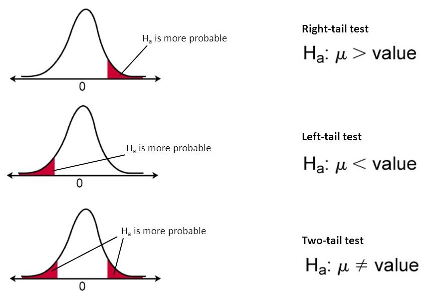
As before, take a statistical test $t$ and data $D$ sampled from some $P(x \mid \theta)$. Let $H_0: \theta = \theta_0$ be the null hypothesis and $H_a: \theta =\theta_a$ the alternative hypothesis. In order to know which hypothesis to reject given some test result, we may endow the test with a rejection region $R$ — whenever $t(D)$ is in this region, we reject $\theta_0$, accepting it (and thereby rejecting $\theta_a$) whenever $t(D)$ is not in $R$. Usually, these rejection regions come in one of two forms:

1. $R = \{x \in \mathbb R \mid x > c\}$ for some $c$, or, symmetrically, $R = \{x \in \mathbb R \mid x < d\}$. Tests with these rejection regions yield rejections of the null hypothesis when their values are above (resp. below) the pre-determined values $c$ (resp. $d$).
   Because the rejection region is in either case a single wing of the real line, these are commonly called one-tailed tests, this tail either being on the left ($x < d$) or the right ($x > c$).
2. $R = \{x \in \mathbb R \mid |x| > e\}$ for some $e$. A test with this rejection region yields a rejection of the null hypothesis when its value is above $e$ or below $-e$.
   Because the rejection region lies on both sides of the real line, these are commonly called two-tailed tests.

Neyman and Pearson's strategy was to, by controlling the boundaries of the rejection regions (the values of $c, d$, and $e$ in the above sets), control the probabilities of type I and type II errors. By convention, they referred to the type I error, or false positive rate, of a given test as $\alpha$. The type II error, or false negative rate, is referred to as $\beta$. Let's define these formally: $$\alpha = P(\text{Type I Error}) = P(t(D) \in R \mid \theta = \theta_0)\qquad \beta = P(\text{Type II Error}) = P(t(D) \notin R \mid \theta = \theta_a)$$

Power

The only way to get a test with no chance of a false positive, $\alpha = 0$, is to always accept the null hypothesis, which forces $\beta = 1$; conversely, the only way to get a test with no chance of a false negative, $\beta = 0$, is to always reject the null hypothesis, which forces $\alpha = 1$. It's clear that we must develop some way to characterize the tradeoff between $\alpha$ and $\beta$.

!tab Neyman and Pearson's approach to this was to first fix some $\alpha$, say $\alpha = 0.05$, and then find a test that minimized $\beta$ while maintaining that $\alpha$. To this end, they introduced the concept of power. The power of a test is the probability that it will reject the null hypothesis when that is the right thing to do. $$\operatorname{Power} = P(t(D) \in R \mid \theta = \theta_a) = 1 - P(t(D) \notin R \mid \theta = \theta_a) = 1-\beta$$

!tab Since the power of a test is simply $1-\beta$, this isn't exactly a new concept — but minimizing $\beta$ is equivalent to maximizing $1-\beta$, which allows us to rephrase the question in terms of finding a most powerful test for some given $\alpha$. The lingo for such a test is an “$\alpha$-level most powerful” test.

!tab P-values are still legible in the Neyman-Pearson framework, since we can still speak of the probability of getting a test result more extreme than an observed one. However, the p-value is no longer the important criterion — the rejection region is. If the p-value isn't at least as small as the fixed $\alpha$, we won't reject, since the test statistic won't have been extreme enough to hit the rejection region, but even when it is, we'll still report the chance of error of our procedure as $\alpha$, even if the p-value is absolutely microscopic.

!tab Neyman and Pearson's justification for this inflexible protocol was given in the form of a frequentist principle they propounded, which is reproduced in this paper: “In repeated practical use of a statistical procedure, the long-run average actual error should not be greater than the long-run average reported error”. If we stick with reporting an error rate of $\alpha$, then our actual error rate should be no greater than our reported rate, whereas if we play fast and loose with p-values, which are not error rates per se, we may end up violating this principle.

The Neyman-Pearson Lemma

As mentioned, the Neyman-Pearson approach relies on selection of a test endowed with a rejection region such that (a) the false positive rate $\alpha$ of the test is equal to some predetermined value, and (b) the false negative rate $\beta$ of thes test is as low as possible — equivalently, the power $1-\beta$ is as high as possible.

!tab Remarkably, they managed to find the general form of such $\alpha$-level most powerful tests, an achievement that considerably bolstered their position by rendering it practical. Their result, known as the Neyman-Pearson lemma, goes like this: for a distribution $P(x \mid \theta)$ and null and alternative hypotheses $H_0: \theta = \theta_0,\ H_a: \theta = \theta_a$, the test statistic and rejection region of the $\alpha$-level most powerful test $t$ is given by $$t(D) := \frac{{\mathcal L}(\theta_0 \mid D)}{{\mathcal L}(\theta_a\mid D)}\quad \quad R = \left\{x \in \mathbb R \mid x > \eta\right\} $$

Here, ${\mathcal L}(\theta_0 \mid D)$ is the likelihood function, equal to $P(D \mid \theta_0)$; we rewrite it to emphasize that it is a function of $\theta$ rather than $D$, and that it is not a probability distribution over $\theta$. The number $\eta$ is chosen so as to make the false positive rate equal to the pre-specified $\alpha$ — the calculation has to be done on a case-by-case basis.

💡 Neyman-Pearsonian statistics seeks to devise methods that can form decisive conclusions from data with controllable error rates.

The Neyman-Pearson/Fisher Debate

As mentioned, the debate between Neyman-Pearson and Fisher was very ferocious and very drawn-out, with both sides slightly updating their positions over the years in ways that make the debate hard to follow without studying the full history. Since we don't have time for that, I'll try to sketch the main points of each side.

My two primary sources for this section are:

• Lehmann's “The Fisher, Neyman-Pearson Theories of Testing Hypotheses: One Theory or Two?” (link)
• Lenhard's “Models and Statistical Inference: The Controversy Between Fisher and Neyman-Pearson” (link)

Critique of Fisherian Testing

P-values aren't frequentist error rates

It's possible to construct situations in which reported $p$-values violate the aforementioned frequentist principle about making sure reported error never exceeds actual error in the long run. I'll construct such a situation in the indented section below; as far as I know this construction is original, though you can skip it and get straight to the punchline.

!tab Suppose that I generate $n$ samples from ${\mathcal N}(0, 1)$ and $n$ more samples from ${\mathcal N}(m, 1)$. I give you one of these sets at random, affirm that it's normally distributed with variance $1$, and ask you to check that the mean is $0$, masking the fact that it may not be $0$. You set up your $z$-test with null hypothesis $H_0: \mu = 0$. Half the time, your $z$-value is going to be randomly sampled from ${\mathcal N}(0, 1)$. The other half of the time, it's going to be distributed as ${{\mathcal N}}(m\sqrt n, 1)$. In both cases, the $p = 0.05$ marker will be at $|z| = 1.96$.

Suppose now that your test does come up as $p < 0.05$. The probability of this happening is given by $$P(p < 0.05) = P(p < 0.05 \mid \mu = 0)P(\mu = 0) + P(p < 0.05 \mid \mu = m)P(\mu = m)\\ = 0.025 + \frac12F(-1.96) + \frac12(1-F(1.96)) = 0.525 + \frac12\left(F(-1.96)-F(1.96)\right)$$ where $F$ is the cumulative distribution function for ${{\mathcal N}}(m \sqrt n, 1)$. What is the probability that $H_0$ is true? $$P(\mu = 0 \mid p < 0.05) = \frac{P(p < 0.05 \mid \mu = 0) P(\mu = 0)}{P(p < 0.05)} \\= \frac{(0.05)(0.5)}{0.525 + \frac12\left(F(-1.96)-F(1.96)\right)} = \frac{0.05}{1.05 + F(-1.96)-F(1.96)}$$ If $m = \frac12$ and $n = 5$, this probability will be $0.199$. So, even if you set your threshold for rejecting the null hypothesis at $p < 0.05$, in the long run $20\%$ of your rejections will be wrong! By tailoring $m$ and $n$ we can make this percentage lie anywhere between $\frac{0.05}{1.05} \approx 4.8\%$ and $50\%$.

!tab Hence, the use of $p$-values alone violates the aforementioned frequentist principle: the reported error rate can be much greater than the actual error rate in the long run. This is why we cannot treat $p$-values as false positive rates, and why we need an alternative hypothesis to calculate the false positive rate with respect to if we are to report error rates.

No clear test to use

To test a hypothesis $\theta = \theta_0$, we need a test statistic $t$ for the assumed underlying distribution $P(x \mid \theta)$. Which statistic should we use, though? Different statistics undoubtedly have different distributions, which may lead us to make different inferences even at the same $p$-value thresholds. The Neyman-Pearson approach answers in terms of power: we should choose the test $t$ that maximizes power, the probability of rejecting the null hypothesis when the alternative is true. They even specified the form of such a test via their lemma. Hence, the Neyman-Pearson approach has a clear way to choose a test; Fisher's approach does not.

💡 Fisherian statistics has no real way to control error rates, since p-values can not be treated as error rates, and it offers no clear way to determine whether one test is better than another for a given purpose.

Critique of Neyman-Pearson Testing

Error values are inflexible

The false positive rate $\alpha$ is the rate at which we reject a true null hypothesis. Because it does not depend on the alternative hypothesis, only the rejection region of the test, we can calculate it without reference to any alternative hypothesis. If you design a test with $\alpha = 0.05$, and end up rejecting the null hypothesis, the Neyman-Pearson framework advises you to report your possible error as $0.05$, because that's the overall probability of incorrectly rejecting the null hypothesis.

!tab As intuitive as this rule is, it can sometimes lead to nonsensical behavior. If we suppose that the men from some tribe in the Amazon rainforest are all tightly clustered around an average height of 5'3” — making this the null hypothesis — only to pick twenty men at random and find that they're all over 7'0”, we can be sure that the chance of this being a false positive is well under $0.05$. Nevertheless, if our original test was made to have $\alpha = 0.05$, that's what we'd have to report as the chance of a false positive. Of course, the $p$-value of this finding — the chance that we'd get twenty goliaths in a row when the average truly is clustered tightly around 5'3” — is as astronomically small as it should be. Not all rejections are the same, and the Neyman-Pearson approach to error reporting is too inflexible to handle this.

!tab The most obvious way to fix this — to report not the predetermined false positive rate of the test but the probability of the null hypothesis producing a result at least as outrageous as yours — simply reproduces $p$-values, which we have already shown cannot be treated as error rates. The second most obvious way to fix this by finding the probability of the null hypothesis conditional on the test statistic, but that boils down to the Bayesian method. This is a genuinely difficult problem.

No clear alternative to use

A null hypothesis is merely a proposition about a single value, and we can perform one of a great many tests to find evidence in favor of this proposition. Neyman and Pearson demand that we select a test to use based on power, but power, being the probability that a test rejects the null hypothesis given that the alternative hypothesis is true, depends on a particular choice of alternative hypothesis $H_a$. If you pick a different $H_a$, you get a different formula for power, and therefore have to pick a different test. It follows that, as Senn puts it here, “[test] statistics are more primitive than alternative hypotheses and the latter cannot be made the justification of the former”. Neyman and Pearson have simply shifted the ambiguity from choice of test to choice of alternative hypothesis.

!tab Fisher's main critique to the use of alternatives came from his experience with the way actual science was done at the time. His contention was that in any given experiment the experimenter knows what they are looking for, and which hypothesis they want to test; all the experimenter needs is a way to tell whether they should take notice of some data that is anomalous with respect to their hypothesis. Why complicate things unnecessarily by throwing in a second hypothesis?

💡 Neyman-Pearsonian statistics has us throw out clear conclusions in order to maintain an inflexible long-term error rate, and only manages to shift the Fisherian ambiguity re testing to a new ambiguity re alternative hypotheses, rather than eliminating ambiguity.

The Point of Statistics: Inductive Inference or Inductive Behavior?

Both Fisher and Neyman-Pearson saw their fundamental disagreement as one over the role of statistical testing. As Mayo explains in her 1985 “Behavioristic, Evidentialist, and Learning Models of Statistical Testing” (pdf), the Neyman-Pearsonian model views the point of statistical testing as providing rules for behavior — namely, the acceptance and rejection of hypotheses — which help prevent us from making errors too often in the long run. Their viewpoint is commonly called inductive behavior.

!tab Fisher, however, strongly believed that the process of actual decision-making could not be mathematized away, since it relied on a whole universe of scientific intuition, pragmatic constraints, and, most importantly, an understanding about the scope and applicability of the model. It was, Fisher argued, the role of the statistician to mediate between the statistical model and the thing it is modelling, using the model as an aid to determine how much evidence some data provides for some belief; this viewpoint is known as inductive inference.

!tab Hence, their debate hinges on their differing interpretations of statistical inference — is it meant to guide us in our decisions, or is it meant to help us interpret the evidence provided by the data? Unfortunately, this aspect of the debate — if not the very content and existence of the debate — has been elided by most instructional textbooks, as historicized by Halpin and Stam in their 2006 “Inductive Inference or Inductive Behavior: Fisher and Neyman: Pearson Approaches to Statistical Testing in Psychological Research” (pdf).

Exploratory Data Analysis

Of course, there are other interpretations. The most popular of these is Tukey's exploratory data analysis (EDA), a method developed in the 60s and 70s that emphasizes exploratory analysis of the data in order to figure out how to model it and what hypotheses to test, thereby “letting the data speak for itself”. To this end, he either invented or popularized many tools for getting a qualitative look at the data without having a model in mind, as described on his Wiki page. This decisively contradicts Neyman-Pearson's behavioral approach, but only mildly concords with Fisher's evidential approach, as Tukey was even more bearish than Fisher on the validity of any particular model. Through exploratory data analysis, statistics is explicitly interpreted as another tool for dialectically building a scientific nature of understanding.

!tab The error of choosing an inappropriate model has been called an “error of a third kind”, in a humorous continuation of Neyman-Pearson's errors of the first and second kinds. We shall have more to say about model selection later, after we've introduced the Bayesian approach to statistical inference.

!tab Of course, when there is a scarcity of data, looking at what data you do have in order to formulate hypotheses will result in hypotheses that are far more likely to apply to your data than to the population, since you came up with those hypotheses specifically in response to that data; this is known as the problem of post hoc theorizing. Better to come up with hypotheses on a limited set of data and see if they extrapolate to the rest of the data. Sometimes it's extremely hard to obtain extra data, in which case we're just kinda screwed; Tukey called this kind of situation “uncomfortable science”.

💡 The Fisher/Neyman-Pearson debate is, at its core, a question over the purpose of statistics; alternative interpretations, such as exploratory data analysis, have been proposed, but have their own issues as well.

A Curious Note: Fiducial Inference

One way that frequentists reason about the parameter $\theta$ underlying some probability distribution $P(x \mid \theta)$ is to construct confidence intervals for $\theta$: a confidence interval for $\theta$ with fixed confidence level $c$ consists of a pair of statistics $s_c, t_c$ of $x$ such that $P(s_c(x) < \theta < t_c(x)) = c$.

!tab At first glance it might seem like this probability concerns the distribution of $\theta$, but it does not: being frequentists, we do not view $\theta$ as having a probability distribution. It just has a value, and correspondingly it is either in the interval or not. The long-run frequency in which it will be in the interval corresponding to the $x$ sampled on any given trial is given by $c$. (Since Bayesians take probabilities to be beliefs, they can form a distribution over $\theta$ — they understand that it is fixed, they're just not certain about where it's fixed, and as such their beliefs as to the location assemble into a probability distribution. Their version of the confidence interval is known as the credible interval).

!tab One of Fisher's stranger statistical ideas was the use of these confidence intervals to form a distribution over the parameter $\theta$ itself. Prima facie, this distribution will depend on the sampled data, since we have to calculate the statistics somehow, but there is a way around this — there are certain functions of the data, known as pivotal quantities, the distributions of which do not depend on $\theta$, even though the data is sampled from $P(x \mid \theta)$. We saw one example of this with the $z$-score: if $D= \{d_1, \ldots, d_n\} \sim {\mathcal N}(\mu, \sigma^2)$, the value $z = \frac{\overline D - \mu}{\sigma/\sqrt{n}}$ is distributed as ${\mathcal N}(0, 1)$. This distribution is independent of the parameters $\mu, \sigma^2$, making $z$ a pivotal quantity. Note that this pivot is not a statistic — a statistic does not directly depend on the parameters of the distribution, whereas $z$ explicitly depends on $\mu$ and $\sigma$.

Fisher's so-called fiducial approach is as follows: first, find $a, b$ such that $P(a < \frac{\overline D - \mu}{\sigma/\sqrt n} < b) = \alpha$ — since the middle term is the $z$-value, this is simple. Now, rearrange as follows: $${\small \alpha = P(a < \frac{\overline D - \mu}{\sigma/\sqrt n} < b) = P(\frac{a\sigma}{\sqrt n} < \overline D - \mu < \frac{b\sigma}{\sqrt n}) =P(\overline D - \frac{b\sigma}{\sqrt n} < \mu < \overline D - \frac{a\sigma}{\sqrt n})}$$

Having moved to the equivalent expression on the right-hand side, we now treat the statistic $\overline D$ as fixed, and the parameter $\mu$ as variable, using this rearrangement to find the probability that $\mu$ lies within some region. This is known as the fiducial probability distribution of $\mu$.

!tab Obviously, by treating $\mu$ as variable, Fisher made an enemy of many frequentists, who conceptualized $\mu$ as a fixed constant already existing in the world. He may have gotten away with this if not for the fact that this approach was also mathematically unsound at best: it has been shown that this does not actually generate a probability distribution on $\mu$, because additivity does not necessarily hold, and even Fisher himself admitted that “I don't understand yet what fiducial probability does. We shall have to live with it a long time before we know what it's doing for us”. As such, fiducial inference didn't get very far, lasting only as a curious footnote in the history of statistical inference.

Likelihoodism

Likelihoodism is a school of statistical inference that can neither be described as frequentist nor as Bayesian. As the name suggests, it focuses on the use of the likelihood function ${\mathcal L}(\theta \mid D) := P(D \mid\theta)$; likelihoodists claim that all evidence that $D$ provides about $\theta$ is contained within this function, a claim known as the likelihood principle. The Neyman-Pearson lemma provides some modest support for the likelihood principle, since it states that the most powerful hypothesis test at any given level is precisely the quotient of the likelihoods of the two hypotheses with respect to the sample data.

Birnbaum, in his 1962 “On the Foundations of Statistical Inference” (pdf), actually derives the likelihood principle from two simpler principles, which I'll paraphrase here (the actual paper being rather obtuse):

• The principle of sufficiency: If an experiment $E$ is divided up into several subcomponents $\{E_\lambda\}_{\lambda \in \Lambda}$, such that $\lambda$ is an ancillary statistic of some distribution and each $E_\lambda$ has its own set of outcomes, then observing outcome $x^\lambda_i$ of experiment $E_\lambda$ provides exactly as much evidence about the underlying distribution as does observing outcome $x^\lambda_i$ of experiment $E$, without knowing that it comes from $E_\lambda$.
• The principle of conditionality: If $t$ is a sufficient statistic for some parameter $\theta$, and two experiments $E_1$ and $E_2$ yield outcomes $x_1$ and $x_2$ such that $t(x_1) = t(x_2)$, then the evidence about $\theta$ provided by each of the two experiments is the same.

Birnbaum argues that the likelihood principle is true if and only if both of these two principles are true; since he assumes both of them to be obvious, he concludes that he has proved the likelihood principle. Naturally, lots of criticism has been directed at this justification, as explained on the Wikipedia page.

Bayesian Inference

Bayesian Testing and Estimation

For the Bayesian, most of the above issues are sidestepped: probabilities are beliefs, and given a model $P(x \mid \theta)$, a prior $P(\theta)$ gives us a degree of partial belief for every possible hypothesis. Given some data $D$, we know exactly how to update our beliefs in these hypotheses: $$P(\theta = \theta_0 \mid D) = \frac{P(D \mid \theta =\theta_0) P(\theta_0)}{\int_{\Omega} P(D \mid \theta = \theta_1)P(\theta_1)\, d \theta_1}$$

This is the rational update to make to our belief. We need not confuse ourselves with issues of whether this data is significant or insignificant evidence, whether we have to either reject or accept any particular hypothesis based on the data, or whether we have to commit to any other particular course of action — Bayesian probability is the logic of partial belief, and, by restricting itself to belief, extends to a statistical framework that manages to sidestep many of the issues of Fisherian and Neyman-Pearsonian statistics.

!tab Because the Bayesian framework doesn't introduce much in the way of new machinery, as the frequentist schools do with hypothesis tests, error rates, and so on, we'll almost immediately have to delve right into mathematics to really see what's going on, rather than critiquing this surface-level machinery as we did with the frequentist schools. As such, this section will be highly mathematical.

!tab A note which exemplifies this: in the denominator of the right hand side of Bayes' law, as written above, we've performed an implicit marginalization. This is the process of removing a parameter from a probability distribution by taking the expectation with respect to that parameter. This is a perfectly legitimate process with respect to the laws of probability, and makes intuitive sense: the probability of sampling $D$ is equivalent to the probability of sampling $D$ and having $\theta = \theta_1$ for some $\theta_1$, for $\theta$ must always equal some value. Hence, $P(D)$ should be a summation over all $\theta_1 \in \Omega$ of $P(D, \theta=\theta_1)$. Since $\theta$ is a continuous variable, we must perform an integral: $$P(D) = \int_{\Omega} P(D, \theta=\theta_1)\, d\theta_1 = \int_\Omega P(D \mid \theta = \theta_1)P(\theta_1)\, d\theta_1 = \mathbb E_\theta[P(D\mid\theta)]$$

The only problem with this is that it can be tricky to calculate, since there's no guarantee that this integral is tractable; in such cases, we may have to turn to alternative computational methods such as Variational Bayes or Markov Chain Monte Carlo, both designed to deal with this problem.

!tab At the same time, because it is only a logic of partial belief, it is not naturally suited to many of the tasks that any framework for statistical inference finds itself asked to perform. Hence, if we consider Bayesianism to be analogous to a computer, then Bayesian probability — the framework of priors, conditionalization, and marginalization — is its kernel, the set of tasks it performs natively; Bayesian statistical inference, on the other hand, is analogous to a software suite running on this computer, each program in which uses the language of Bayesian probability to perform tasks well beyond the ambit of Bayesian probability.

I'll give a couple examples of these programs.

Meeting The Demands of Statistical Inference

1. Bayesian estimation: Given some data $D \sim P(x \mid \theta)$ and a prior $P(\theta)$, the classical way that a Bayesian would come up with a single estimate for $\theta$ is to first calculate the posterior $P(\theta \mid D)$, and then to take the mode of this posterior distribution, yielding the estimate $$\widehat \theta(D) := \operatorname{argmax}_{\theta} P(\theta \mid D)$$ (This is an example of an estimator, or a function of the data designed to yield an estimate of some parameter. An estimator of a parameter $\theta$ is generally denoted by $\widehat \theta$, as above).
   The estimator given by the mode of the posterior distribution of the parameter $\theta$ is known as the maximum a posteriori (MAP) estimator for $\theta$. An example of MAP estimation for a normal distribution with known variance and unknown mean is given in Appendix B.5; it turns out to be an elegant weighted average of the sample mean and the mean of the prior placed over the unknown mean $\mu$.
   There are other methods of doing Bayesian estimation, most of which have the following structure:
   1. Construct a loss function $L(\theta_1, \theta_2)$, such as the mean squared error $L(\theta_1, \theta_2) :=(\theta_1-\theta_2)^2$.
   2. Define a corresponding functional $F(\widehat\theta) := \mathbb E_{\theta, D} \left[L(\widehat\theta (D), \theta)\right]$.
   3. Find the estimator $\widehat\theta$ that minimizes this functional.
   If we use mean squared error loss, for instance, the estimator that arises is given by the mean of the posterior distribution, as shown in appendix B.6.


2. Bayesian hypothesis testing: If we really want to get a single number representing the strength of one hypothesis $H_0: \theta = \theta_0$ over another hypothesis $H_a: \theta = \theta_a$, we may calculate the Bayes factor of the two hypotheses. Given some data $D \sim P(x \mid \theta)$, this factor is calculated as $$K := \frac{P(D \mid \theta = \theta_0)}{P(D \mid \theta = \theta_a)}$$ That's it. A value of $K$ over $1$ indicates support for $H_0$, while a value of $K$ under $1$ indicates support for $H_a$. The more extreme this value is, the stronger the evidence; one table commonly used to convert from Bayes factors to qualitative judgements is as follows:
   • $K < 1$ : Negative
   • $1 < K < 3$ : Trifling
   • $3 < K < 10$ : Substantial
   • $10 < K < 30$ : Strong
   • $30 < K < 100$ : Very strong
   • $100 < K$ : Decisive

💡 The Bayesian approach to statistics consists of a bunch of heuristics and rules loosely tacked on to the Bayesian approach to probability; it's more like engineering, and is of questionable philosophical coherence.

The Neverending Search For Objective Priors

The biggest weakness in the Bayesian approach to statistical inference is, as with Bayesianism in general, the generation of priors; this falls prey to the same critiques we discussed in the previous article. As mentioned in that article, it is primarily objective Bayesians who concern themselves with finding priors that could in some sense be considered “canonical”, bringing in no extraneous information; correspondingly, the subfield of Bayesian inference that relies on such priors is objective Bayesian inference. Of course, the grass isn't much greener on the other side: eschewing objectivity in our priors forces us to bring in our own assumptions and biases, thereby skewing our analysis in the best case, and in the worst case forcing this analysis to simply tell us what we already knew.

!tab First, we'll study methods of generating “perfect” objective priors, which bring in absolutely no information. There are at least five ways to do this: use of the principle of maximum entropy to generate a prior, the use of an algorithmic universal prior, calculation of the Jeffreys, reference, maximal data information, or Haar priors, and empirical Bayesian methods for calculating a reasonable prior from some data. We've covered algorithmic universal priors and the principle of maximum entropy previously, so we'll cover the other other five methods here.

💡 Bayesian statistics inherits the objectivity issues of Bayesian philosophy.

Jeffreys, Reference, Maximal Data Information, and Haar Priors

Fisher Information and the Geometry of Parameter Space

For some parametrized probability distribution $P(x \mid \theta)$, the Fisher information of $\theta$ is given by $$I(\theta) := \mathbb E \left[\left(\frac{\partial \ln P(x \mid \theta)}{\partial \theta}\right)^2\right]$$

When there are multiple parameters, $\vec \theta = [\theta_1,\ldots, \theta_n]^T$, we may generalize this to get an $n \times n$ matrix as follows: $$[I(\vec \theta)]_{ij} := \mathbb E \left[\left(\frac{\partial \ln P(x \mid \theta_i)}{\partial \theta_i}\right)\left(\frac{\partial \ln P(x \mid \theta_j)}{\partial \theta_j}\right)\right]$$

This is the Fisher information matrix (FIM). (Clearly, if there's only one parameter, then the FIM is the $1\times 1$ matrix containing the Fisher information of that sole parameter). It is designed to capture a rather intuitive property of the parameter space: changes of some parameters qualitatively affect the distribution more than changes of other parameters, and this relative change depends on the value of the parameters when they are changed, in the same way that the relative change of some function depends on the value of the function at the point that it is changed.

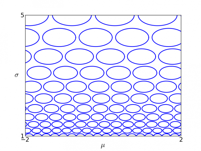
!tab At some fixed parameter vector $\vec \theta_0$, the infinitesimal change in information that an infinitesimal parameter change $d\vec \theta$ will evoke is given by the product $[(d \vec \theta)^T I(\vec \theta_0) (d\vec\theta)]^{-1/2}$, which is a scalar of order $O(||d\vec \theta||)$. This product induces a metric on the tangent space to each point of the parameter space, thereby endowing it with a local geometry.

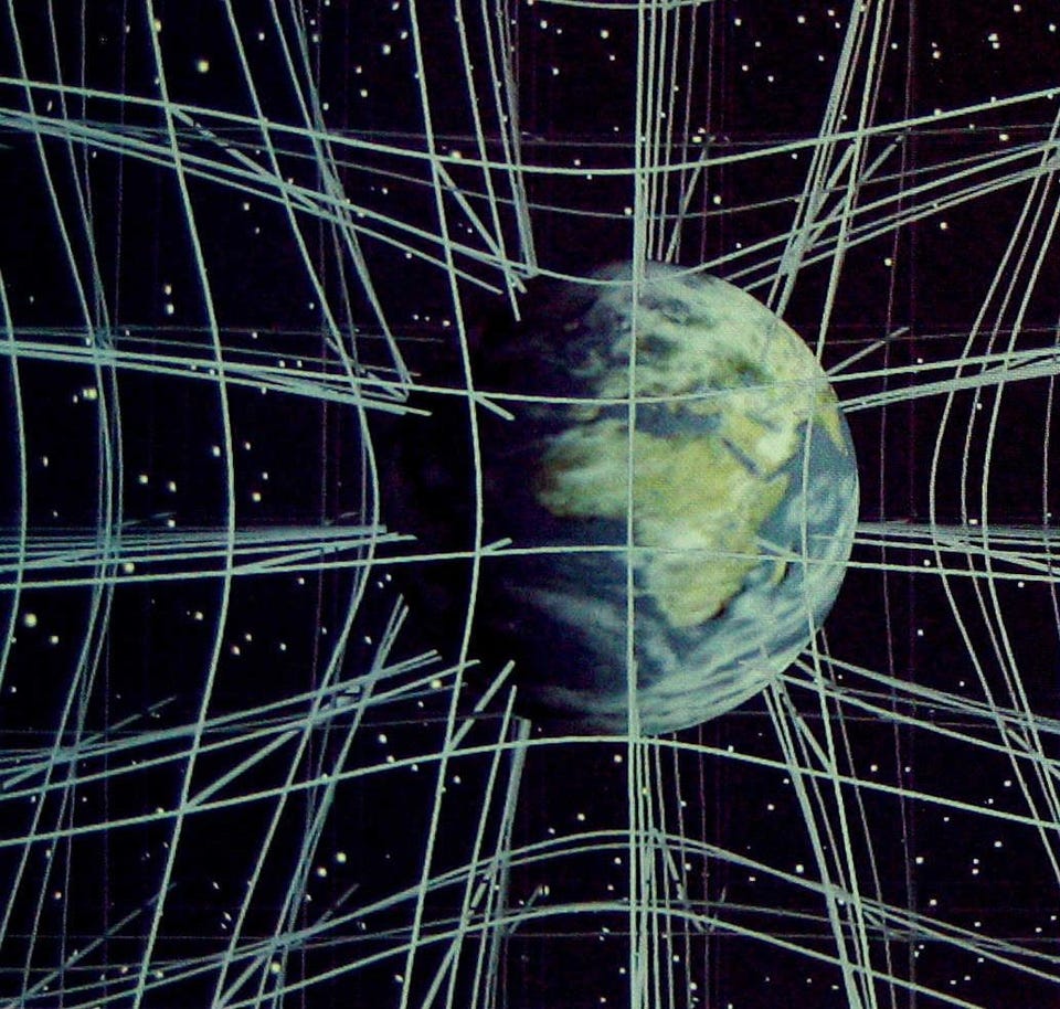
!tab To really understand this notion requires a course in differential geometry, which I'm not going to provide here. The essential idea is that the Fisher information matrix can be used to endow the parameter space with a space-like geometry, complete with curvature and geodesics. This is an extremely powerful idea, and motivates the field of information geometry, the study of such parameter spaces in their geometric aspect. What is relevant for our purposes, though, is that this space has a “local volume” — it stretches and contracts as you move through it, in the same way that the fabric of the universe stretches and contracts (due to the presence of mass-energy). The quantity measuring the amount of stretching at any given point, i.e. the Riemannian volume form, has magnitude $|\det I(\vec \theta)|^{-1/2}$; this magnitude is entirely a property of the local geometry of the space, and remains the same under changes of coordinates.

The Jeffreys Prior

The volume form derived from the Fisher information metric is what is used to define the Jeffreys prior: $$P(\vec \theta) \propto |\operatorname{det} I(\vec \theta)|^{-1/2}$$

It corresponds to a sort of content-aware scaling on the parameter space, and is invariant under reparametrization.

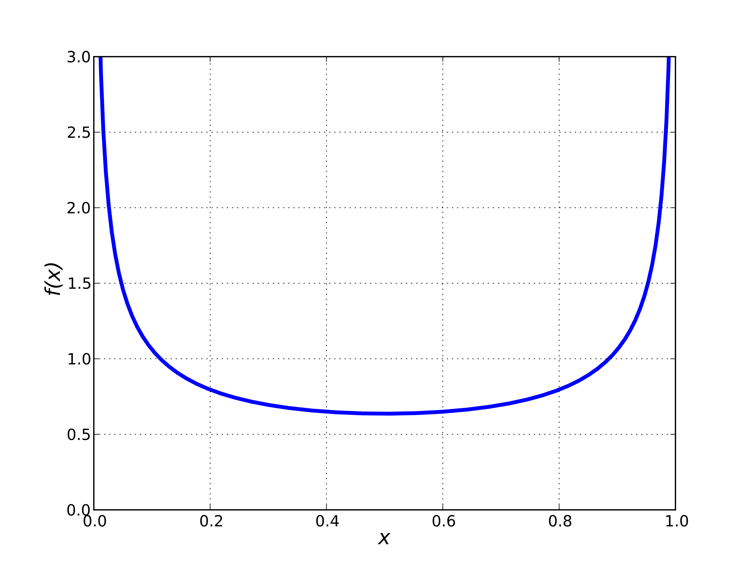
An example: take the Bernoulli distribution $\operatorname{Bern}(p)$, given by $P(x \mid p) = p^x(1-p)^{1-x}$. The Fisher information of this distribution at parameter $p$ is given by $$I(p) = \mathbb E\left[\left(\frac{\partial}{\partial p}(x \ln p + (1-x)\ln(1-p))\right)^2\right] = \sum_{x \in \{0, 1\}} \left(\frac{x}{p} -\frac{1-x}{1-p}\right)^2p^x(1-p)^{1-x} = \frac{1-p}{(1-p)^2} + \frac{p}{p^2} = \frac{1}{1-p}+\frac1p = \frac{1}{p(1-p)}$$

So the Jeffreys prior for $p$ is, prior to normalization, $\sqrt{|I(p)|} = \frac{1}{\sqrt{p(1-p)}}$. This integrates to $\pi$ (Wolfram|Alpha), giving us a normalized prior $P(p) = \frac{1}{\pi\sqrt{p(1-p)}}$. Fortunately, this is precisely $\operatorname{Beta}\left(\frac12, \frac12\right)$, the conjugate prior for the Bernoulli distribution, so we know how to do inference with it. (Since the cumulative distribution function of this distribution is given by $P(X \le x) = \frac2\pi \arcsin(\sqrt{x})$, this is sometimes called the arcsine distribution as well).

Note that this isn't even uniform. However, uniformness is not invariant under reparametrization. If we let our variable be not the per-trial chance of a success but the logarithm of the chance of a success, $\ell = \ln p$, then $P(\ell = x) = \frac{d}{dx} P(\ell \le x) = \frac{d}{dx} P(\ln p \le x) = \frac{d}{dx} P(p \le e^x) = e^x$. This is normalized, since $\ell$ is necessarily negative: $\int_{-\infty}^0 P(\ell) d\ell = e^\ell|_{-\infty}^0 = e^0 - e^{-\infty} = 1$, but it is clearly not uniform. (This is one major problem with uniform distributions: when over infinite sets, they depend on the particular parametrization of the problem. In the previous article, this phenomenon was the cause of Bertrand's paradox: there is no single uniform distribution over chord space, only a uniform distribution over some particular parametrization of chord space).

!tab Unfortunately, there's a reason I had to define the Jeffreys prior as only being proportional to the volume form: Jeffreys priors are often not normalizable. For instance, the Fisher information of the mean of a normal distribution with known variance is given by $I(\mu) = 1/\sigma^2$. The unnormalized Jeffreys prior is therefore $P(\mu) = 1/\sigma$, but this is constant with respect to $\mu$, and therefore $\int_{-\infty}^\infty P(\mu)\, d\mu = \frac1\sigma \int_{-\infty}^\infty d\mu = \infty$.

!tab This is often the case with Jeffreys priors, a terrible drawback to such an elegant method. This issue will repeatedly come up as we explore more methods of generating objective priors, and we shall discuss it in detail later.

Reference Priors

Another strategy to construct a noninformative prior is to take the word “noninformative” literally, and construct a prior whose expected information gain upon conditioning upon some observation is as large as possible.

Typically, the quantity used to measure the change in information effected by moving from one distribution $Q$ to another distribution $P$ is the Kullback-Leibler divergence, defined as $$\operatorname{KL}(P \mid\mid Q) := \int_{-\infty}^\infty P(x)\ln\frac{P(x)}{Q(x)}\, dx$$

To construct this noninformative prior, then, we'll take some some sufficient statistic $t$ and attempt to maximize the information differential between $P(\theta \mid t)$ and $P(\theta)$, which can be expressed in terms of the following integral: $$\mathbb E_t\left[\operatorname{KL}(P(\theta) \mid\mid P(\theta \mid t))\right] = \int P(t)\int P(\theta \mid t) \ln \frac{P(\theta \mid t)}{P(\theta)}\, d\theta\, dt = \iint P(\theta, t) \ln \frac{P(\theta, t)}{P(\theta)P(t)}\, d\theta\,dt$$

The prior $P(\theta)$ that maximizes this value is known as the reference prior for $\theta$. Amazingly, the reference prior for a parameter is often equivalent to the Jeffreys prior for that parameter; less amazingly, this causes reference priors to inherit the non-normalizability problems of Jeffreys priors.

!tab Furthermore, one might question the choice of the Kullback-Leibler divergence. This divergence isn't even an actual metric on the space of probability distributions, since it isn't symmetric; if we were to choose another formula for divergence, of which there are many, we could get a different answer, as shown by Ghosh's “Objective Priors: An Introduction for Frequentists” (pdf).

Maximal Data Information Priors

Given a distribution $P(x)$, the entropy of $P(x)$ is defined by $$H[P(x)] := \mathbb E_{x}[\ln P(x)^{-1}] = -\int_X P(x)\ln P(x)\, dx$$

This is an information-theoretic concept like the KL divergence, though its meaning is a bit tricky. For our purposes, we may consider it as a measure of the information inherent to some distribution. This immediately suggests another way to construct a noninformative prior, in a manner analogous to the construction of the reference prior: given $P(x \mid \theta)$: maximize the sum of the entropy of the prior $P(\theta)$ with the expected entropy of $P(x \mid \theta)$, thereby constructing a prior which is both noninformative and produces a noninformative model. Hence, what we want to maximize is the functional $$F[P(\theta)] = H[P(\theta)] + \mathbb E_{\theta}\left[H[P(x \mid \theta)]\right] \\ = -\int_\Omega P(\theta)\ln P(\theta)\, d\theta - \int_\Omega P(\theta)\int_X P(x \mid \theta) \ln P(x \mid \theta)\, dx\, d\theta$$

The prior that maximizes this functional is known as the maximal data information prior for $\theta$. Often, this yields priors that are different from the above methods: Kass and Wasserman's “The Selection of Prior Distributions by Formal Rules” (pdf) concerningly says of Zellner's method that it “leads to some interesting priors”. Indeed, it seems rather arbitrary to me to sum the entropy of $P(\theta)$ with the expected entropy of $P(x \mid \theta)$.

!tab However, I learned the hard way that this approach falls prey to the same non-normalization problem: after being unable to find the MDI prior for the normal distribution with known mean and unknown variance, I tried calculating it myself (see Appendix B.3), only to find that it was equal to the non-normalizable Jeffreys prior $P(\sigma^2) \propto \sigma^{-1}$. Hence, we get the fatal flaw of the above approaches plus a spoonful of apprehension.

Haar Priors

🚨 Math warning: group theory, measure theory

If we can't construct a probability distribution over a parameter $\theta$ that is invariant under all transformations, as the Jeffreys prior is, perhaps we can construct a probability distribution that is invariant under some collection of specified transformations. Because it makes the theory significantly easier, we assume that these transformations form a group: they are closed under composition, they all have inverses which are all specified transformations, and the identity transformation is a specified translation. Formally, any collection of elements that satisfies these properties (with respect to some notion of composition and inversion) is called a group, and when each of these elements can be considered as a transformation on some set, e.g. the set of probability distributions on $\theta$, we speak of a group action. Nevertheless, if you don't already know group theory, I advise you to skip this section.

!tab The first step in this approach is to take a sample space $X$ upon which a group $G$ acts. If $P(x \mid \theta)$ is a parametrized distribution on $X$, with parameter space $\Omega$, then in certain cases the action of $G$ on $X$ may lift to an action of $G$ on $\Omega$. For instance, if $G$ is the group of affine transformations $x \mapsto ax+b$, and $P$ is ${\mathcal N}(\mu, \sigma^2)$, then, since $P(ax+b \mid \mu, \sigma^2) = P(x \mid a\mu+b, a^2\sigma^2)$, the element $g \in G$ acting on $X$ by sending $x$ to $a x + b$ can be considered to act on $\Omega$ by sending $(\mu, \sigma^2)$ to $(a\mu + b, a^2\sigma^2)$. Let $\overline G$ be the group acting on $\Omega$.

!tab Under certain conditions on $G$, measure theory guarantees the existence of two measures on $\overline G$: the left Haar measure $\mu_L$, which satisfies $\mu(\overline g S) = \mu(S)$ for all measurable $S \subseteq \overline G$ and elements $\overline g \in \overline G$, and the right Haar measure $\mu_R$, which satisfies $\mu(S\overline g) = \mu(S)$. When the lifted group $\overline G$ can be identified with the parameter space $\Omega$, as was the case in the above example, these measures can be identified with measures on $\Omega$, known as the left and right Haar priors.

Kass and Wasserman, linked above, discuss qualitative differences between these priors on pg. 6, and quote a convincing argument by Villegas in favor of the right Haar prior: pick any parameter (set) $\theta$, and define the map $\phi_{\theta}: G \to \Omega$ by $\phi_\theta(g) = g(\theta)$. Any measure $\nu$ on $G$ can be pushed forward by $\phi_\theta$ to a new measure $\mu$ on $\Omega$ given by $\mu_\theta(S) = \nu(\phi^{-1}_\theta(S))$$\mu(S) = \nu(\phi^{-1}_\theta(S)) = \nu(\{g \in G \mid g(\theta) \in S\})$. Suppose that this is invariant under choice of $\theta$. Then, for every $h \in G$ we'll have $\mu_{h(\theta)} = \mu_\theta$. But $\mu_{h(\theta)}(S) = \nu(\{g \in G \mid (gh)(\theta) \in S\}) = \nu(\phi^{-1}_\theta(S)h)$, so we must have $\nu(\phi^{-1}_\theta(S)h) = \nu(\phi^{-1}_\theta(S))$, evidencing the importance of right translation invariance. Villegas finishes this line of thought to prove that this implies that $\mu_\theta$ is the right Haar prior on $\Omega$.

!tab This construction provides one way to get priors on the parameter $\theta$ where other constructions might fail. However, not only does it require many specific conditions and choices — we have to have $G$ locally compact, we have to have an identification of the lifting of $G$ with the parameter space, and we have to choose between a left and right Haar prior, which may not be the same, but it also often fails to yield a normalizable prior in many cases of interest.

!tab For instance, whenever $P(x \mid k, \ell)$ is of the form $\frac{1}{\ell}f((x-k)/\ell)$, the left and right Haar priors for the action $g_{a, b}(x) = ax+b, \overline g_{a, b}(k, \ell) = (ak+b, a \ell)$ are given by $\mu_L(k, \ell) \propto \ell^{-2}$ and $\mu_R(k, \ell) \propto \ell^{-1}$. In particular, this result covers the normal distribution example above, via $k = \mu, \ell = \sigma$ and $f(r)=e^{-r^2/2}/\sqrt{2\pi}$, from which it follows that the left and right Haar priors are given by $P_L(\mu, \sigma^2) \propto \sigma^{-2}$ and $P_R(\mu, \sigma^2) \propto \sigma^{-1}$. Neither of these are normalizable.

The principle of indifference, by the way, can be considered from a group-theoretic standpoint as the only probability distribution on a finite set $X$ of cardinality $n$ that is invariant under the action of $S_n$ (the symmetric group of order $n$), when this group is considered as the group of all bijections $X \to X$.

💡 There are multiple different approaches to constructing “objective” priors — (1) use the inherent geometry of the parameter space, (2) maximize informational distance between prior and posterior, (3) minimize joint information across prior and model, (4) enforce a fixed set of symmetries. These often (though not always) yield the same results, which lends some credence to their “objectivity”; tragically, however, they all tend to generate non-normalizable priors.

Are Non-Normalizable Priors Okay?

We've seen that most of the methods used to generate objective Bayesian priors have the extraordinarily bad habit of generating measures that aren't even probability distributions: they integrate to infinity, and therefore cannot be normalized; these non-normalizable priors are generally called improper. Sometimes, it will be true that the posterior obtained by an improper prior is proper, so that we can go ahead and proceed with inference.

If you ask an objective Bayesian, they'll tell you this is almost always the case: for instance, given a normal distribution with known variance and unknown mean, setting a constant prior over the mean, $P(\mu) = c$, gives us a posterior of $$P(\mu \mid x) = \frac{P(x \mid \mu)P(\mu)}{\int_{-\infty}^\infty P(x\mid \mu)P(\mu)\, d\mu} = \frac{\frac{c}{\sqrt{2\pi\sigma^2}}e^{-\frac12\frac{(x-\mu)^2}{\sigma^2}}}{\int_{-\infty}^\infty \frac{c}{\sqrt{2\pi\sigma^2}}e^{-\frac12\frac{(x-\mu)^2}{\sigma^2}}\,d\mu} = \frac{e^{-\frac12\frac{(x-\mu)^2}{\sigma^2}}}{\int_{-\infty}^\infty e^{-\frac{\mu^2}{2\sigma^2}}\,d\mu} = \frac{1}{2\pi\sigma^2}e^{-\frac12 \frac{(\mu-x)^2}{\sigma^2}}= {{\mathcal N}}(\mu \mid x, \sigma^2)$$

(Note that $x$, not $\mu$, plays the role of the mean in the RHS; the posterior on $\mu$ is a normal distribution with average given by the observed $x$ and variance given by $\sigma^2$). Hence, while these improper priors are not actually proper, if we treat them as talking about the relative likelihood of picking one value over another, then we can have our cake and eat it too by being able not only to interpret them, but to convert them into proper posteriors, giving us true objective priors (modulo the choice of method for generating those priors, at least). However, this does not always happen; an example is given on page 17 of the Kass and Wasserman paper linked above. This not only makes use of methods that can generate improper priors unsuitable for general use, but makes us question their coherence in general.

💡 Non-normalizable (improper) priors are sometimes okay, in the sense that they often generate proper posteriors; they do not always do so, though, which brings into question the coherence of any method that generates them.

Empirical Bayesian Methods

These methods, unlike the previous ones, give us a way to construct prior propers. As usual, we have data $D$ drawn from a distribution $P(x \mid \theta)$, and the question is the generation of a prior $P(\theta)$. Let's assume that this prior is itself parametrized (e.g., as a conjugate prior is), as $P(\theta \mid \gamma)$ — here $\gamma$ is a hyperparameter. Our previous approaches to generating a prior that incorporates no additional information have failed: the maxentropy and Jeffreys priors either don't exist or are clearly useless (e.g., as a normal distribution ${\mathcal N}(0, 1)$ would be useless to model the mass of the sun in kilograms), and universal priors like the Solomonoff would be intractable if we even knew how to specify them precisely in the situation at hand.

!tab Empirical Bayes attempts to construct the prior $P(\theta \mid \gamma)$ from scratch using the observed data $D$, using as little extra information as possible, by choosing the $\gamma$ that maximizes $P(D \mid \gamma) = \int P(D \mid \theta)P(\theta \mid \gamma)\, d\theta$.

An example: suppose I wanted to figure out the rate of spam emails I'll get next week, having gotten 50 this week and 75 last week. Since these spam emails are sent (for the most part) independent of one another, I can say that these numbers are the result of spam emails coming in randomly at some rate $\lambda$.

!tab I can model this rate with a Poisson distribution $\operatorname{Pois}(\lambda)$: given a non-negative integer $k$, $P(k \mid \lambda)$ is the chance that I'll receive $k$ spam emails in a week given that their rate paces out $\lambda$ spam emails in a week. This value is equal to $(\lambda^ke^{-\lambda})/k!$. What we're looking for is a prior over $\lambda$. The conjugate prior here is the Gamma distribution $\operatorname{Gamma}(\alpha, \beta)$, given by $$P(\lambda \mid \alpha, \beta) = \frac{\beta^{\alpha}\lambda^{\alpha-1}e^{-\beta\lambda}}{\Gamma(\alpha)}$$

We want to use our data $D = \{75, 50\}$ to find the most likely values of $\alpha$ and $\beta$. As mentioned, we'll attempt to do this by maximizing $P(D \mid \alpha, \beta)$. I've shown in Appendix B that this results in $\alpha/\beta$ being set equal to the sample mean, but I can't solve for $\alpha$ and $\beta$ individually (and I tried for hours); there might not be a closed-form solution (or I might just be stupid?). It can be solved numerically, in any case, giving us a prior that does not incorporate additional information. One drawback, however, is that our prior already incorporates the data itself, which is not what priors are supposed to do.

!tab There are many nonparametric approaches to empirical Bayesian estimation, which do slightly better morally by placing no assumptions on the nature of the hyperprior; these often work by finding a hyperprior that minimizes some loss functional derived from the data, such as the Kiefer-Wolfowitz nonparametric maximum likelihood estimator. However, these tend to be significantly more difficult to calculate, either theoretically or numerically.

💡 Empirical Bayesian methods allow for the generation of truly proper priors that don't incorporate information beyond the data, at the cost of “double-dipping” from the data.

Conclusion

All known schools of statistical inference suffer from severe flaws: frequentist schools from an inability to properly handle error and ambiguities in the choice of tests/hypothesis, and Bayesian schools from a lack of canonical solutions to several problems that statistics is expected to perform and a difficulty consistently generating objective priors. These flaws are greatly exacerbated by the fact that statisticians, both in practice and pedagogy, cover such foundational issues with all the vigilance of a dead rabbit; the most famous example of this is the near-universal misuse of the p-value, a subtle idea which the rank-and-file statisticians driving science are simply not equipped, let alone incentivized, to properly interpret and apply.

!tab As with probability, then, it seems that the only option that we have for now is to contextualize our statistical inferences by investigating and clarifying the purpose of our investigations, the rationale for our modeling and testing decisions, and the interpretation of the various numbers we're dealing with. It is so easy to fall into error for any one of a myriad of reasons each of which is invisible to us until it blows up in our face, but paying attention to foundational issues will at least serve as a prophylactic against error — not a cure, since many errors arise from incompatibilities in deeply held, often subconscious commitments to certain ideas about the ontology of the world and the nature of its entities — but at least a prophylactic.

Appendix A. Common Distributions

1. The Normal and Log-Normal Distributions

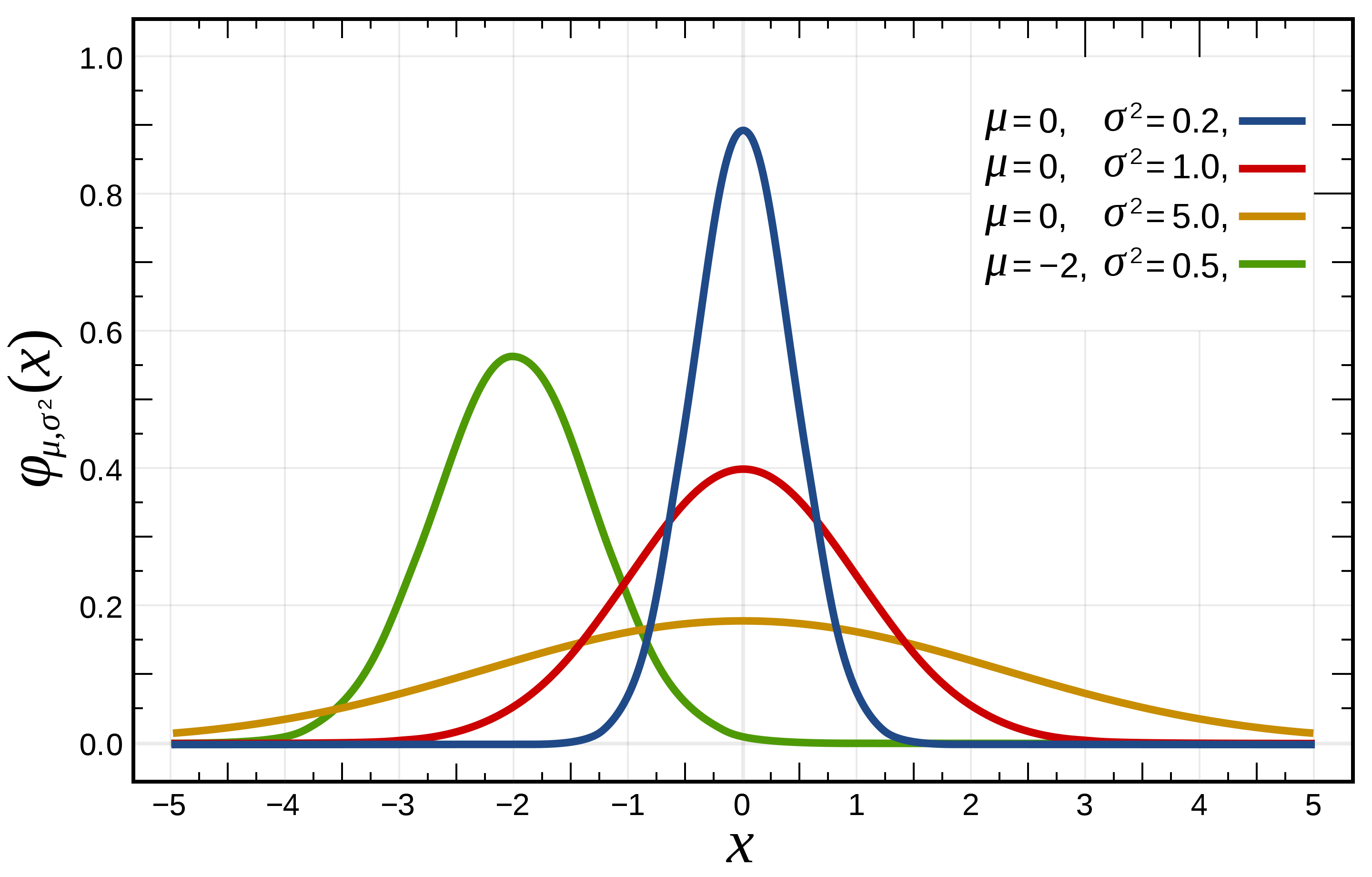
Also called the Gaussian distribution due to its discovery by Carl Friedrich Gauss, the normal distribution is so-called due to its ubiquity in the empirical sciences. The normal distribution $\cal N(\mu, \sigma^2)$ is defined in reference to a mean $\mu$, around which normally distributed samples will congregate symmetrically, and a variance $\sigma^2$, denoting the average squared distance of a sampled point from the mean.

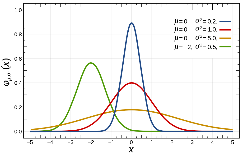
The normal distribution $\cal N(\mu, \sigma^2)$ can be defined as the distribution with the maximum entropy among all distributions with mean $\mu$ and $\sigma^2$. As Wikipedia demonstrates, this alone allows us to find its PDF: $$p(x) = \frac{1}{\sqrt{2\pi\sigma^2}} e^{-\frac12 \frac{(x-\mu)^2}{\sigma^2}}$$

The main reason for the ubiquity of the normal distribution is the central limit theorem, which states that if we have a method of drawing random samples from one underlying population in an independent manner (the idiosyncratic way of saying this is “independent and identically distributed” random variables), then the mean of these samples will converge to a normal distribution. Namely, suppose that we call the $m$th draw from this population $X_m$, and let $S_n = \sum_{i=1}^n X_i$ be the $n$th partial sum. If the mean of the population is $\mu$ and the variance is $\sigma^2$, $S_n$ will converge to $\cal N(n\mu, n\sigma^2)$ as $n$ grows large. For instance, suppose each $X_i$ represents a fair coin flip, $X_i = 0$ if tails and $1$ if heads. The mean of the infinite population of “possible” coin flips is $1/2$, while the variance is $1/4$. As such, the probability distribution of the sum of $n$ coin flips will, as $n$ grows large, converge to the normal distribution with mean $n/2$ and variance $n/4$.

This isn't the sort of case where the conditions have to be just right for the sampled sum distribution to approximate the normal distribution — this happens in a very wide variety of cases, even when the $X_i$ are neither independent nor identically distributed. It results in the general $e^{-x^2}$ term appearing in a wide variety of models of empirical processes.

For instance, in Brownian motion, an atom is jostled around randomly by other atoms with no preferred direction. Each jostle can be thought of as a single random movement of the atom along some arbitrary axis, with mean zero (since no preferred direction) and variance $v$ in inches squared; if there are $r$ collisions per second, then after $t$ seconds there are $rt$ collisions, and we can expect the location of the particle along the given axis to be distributed as $\cal N(0, rtv)$. In other words, if we place some marked atoms at a fixed point in a solution where they're subject to Brownian motion, then after $t$ seconds we should expect them to have spread out in a circle with a density distribution matching the normal distribution along any particular axis. This is exactly what we see, as per the diffusion equation.

The Log-Normal Distribution

Often, we have a large amount of independent variables being multiplied rather than added; since the logarithm of the product of a set of random variables is the sum of the logarithms of the individual random variables, the CLT may tell us how these large products tend to look.

Suppose we sample some numbers $X_1, \ldots, X_n$ from a fixed random variable $X$ and multiply them. $\prod_{i=1}^n X_i = \operatorname{exp}\left(\sum_{i=1}^n \ln X_i\right)$, so if $\ln X$ has mean $\mu$ and variance $\sigma^2$, $\sum_{i=1}^n \ln X_i$ will as $n$ grows large converge to a normal distribution with mean $n\mu$ and variance $n\sigma^2$. It follows that the distribution of the product of the $X_i$ is the exponential of a normal distribution. A distribution which is the exponential of a distribution with mean $\mu$ and variance $\sigma^2$ is known as the log-normal distribution on $\mu$ and $\sigma^2$, or $\operatorname{LN}(\mu, \sigma^2)$

The expected value of the exponential of some $X \sim \cal N(\mu, \sigma^2)$ is $e^{\mu + \sigma^2/2}$, so the mean of $\operatorname{LN}(\mu, \sigma^2)$ will be $e^{\mu + \sigma^2/2}$. The most notable property of the log-normal distribution is its extremely long tail: the mean of $\operatorname{LN}(0, 4^2)$ is $e^8\approx 2981$, but the one in a hundred level is 11 thousand, the one in ten thousand level is 2.9 million, and the one in a million level is 180 million. These distributions and their long tails show up wherever processes are mediated by many multiplicative factors; Wikipedia gives an impressive list.

2. The Bernoulli and Binomial Distributions

Unlike most other distributions we've talked about, these distributions are strictly over the natural numbers: they assign probabilities to 0, 1, 2, and so on.

The Bernoulli Distribution

The Bernoulli distribution is perhaps the simplest possible nontrivial distribution: $\operatorname{Bern}(p)$ is defined as the distribution on {0, 1} sending $1$ to $p$ and $0$ to $1-p$. Conceptually, we often consider this as representing the outcome of a probabilistic trial with exactly two outcomes (or, a Bernoulli trial). For instance, if a coin has a 75% chance of landing heads, then sending heads to $1$ and tails to $0$ allows us to consider this coin as having a $\operatorname{Bern}(0.75)$ distribution. Algebraically, we may write: $$P(x \mid p) = p^x(1-p)^{1-x}$$ As expected, $P(0 \mid p) = p^0(1-p)^{1-0} = 1-p$, while $P(1 \mid p) = p^1(1-p)^{1-1} = p$. The mean of $\operatorname{Bern}(p)$ is simply $$\mathbb E[x] = \sum_{x \in \{0, 1\}} x P(x \mid p) = 0(1-p) + 1(p) = p$$ while the variance is $$\mathbb E[(x-\mu)^2] = \sum_{x \in \{0, 1\}}(x-p)^2P(x \mid p) = (0-p)^2 (1-p) + (1-p)^2p \\ = p^2 - p^3 + p - 2p^2 + p^3 = p(1-p)$$

The Binomial Distribution

Sum up $n$ Bernoulli trials and you get a distribution representing the number of successes in $n$ identical trials each with probability $p$ of success. This is known as the binomial distribution $\operatorname{Bin}(n, p)$. The probability of getting $k$ successes out of $n$ trials is going to be a sum over the probabilities of all possible ways of getting $k$ successes.

Take $n = 100$. The probability of getting $2$ successes in $100$ trials is the same regardless of whether those successes are on trials #1, #2, and #3 or trials #21, #44, and #87. Since the trials are independent, each of these runs has a probability given by $p \times p \times (1-p) \times (1-p) \times \ldots \times (1-p) = p^2(1-p)^{100-2}$. However, there are many more ways to get $2$ successes than there are ways to get $1$ success: there are $100$ ways to pick one number between $1$ and $100$, while there are $100 \times 99 / 2 = 4950$ ways to pick two numbers between $1$ and $100$, disregarding order. In general, the number of ways to pick $k$ numbers out of $n$ will be given by the binomial coefficient $$\binom nk = \frac{\overbrace{n \times \ldots \times (n-k+1)}^{\text{pick } k \text{ different numbers}}}{\underbrace{k \times \ldots \times 1}_\text{regard same choices with different orders as identical}} = \frac{n!}{k!(n-k)!}$$ Hence, the total probability of getting $k$ successes out of $n$ trials will be given by $$P(k \mid n, p) = \binom nk p^k(1-p)^{n-k}$$ By the binomial theorem, this is already normalized: $$1 = 1^n = (p+(1-p))^n = \sum_{k=0}^n \binom nk p^k(1-p)^{n-k} = \sum_{k=0}^n P(k \mid n, p)$$ The mean and variance of $\operatorname{Bin}(n, p)$ are $np$ and $np(1-p)$, though proving this directly from the definition requires some combinatorial trickery.

The fact that $\operatorname{Bin}(n,p)$ is the sum of $n$ Bernoulli distributions allows us to pull an interesting trick: for $n$ large enough, the Central Limit Theorem implies that this sum will converge to a normal distribution with mean $np$ and variance $np(1-p)$. In practice, the normal approximation $\operatorname{Bin}(n, p) \approx {\cal N}(np, np(1-p))$ is acceptable when $np$ and $n(1-p)$ are both above some particular value, such as $9$.

3. The Chi Squared Distribution

Pearson's $\chi^2$ test is a statistical test for determining whether a set of empirical frequencies $e_1, \ldots, e_n$ within some population differs significantly from a set of theoretical frequencies $t_1, \ldots, t_n$. In other words, it measures the “goodness of fit” of the empirical frequencies to the theoretical frequencies. (Note: this Pearson is Karl Pearson, not the Egon Pearson forming the Neyman-Pearson duo. Not a coincidence, though — Karl was Egon's father).

For instance, suppose you show me an ocean of evenly mixed jellybeans, assuring me that 60% of them are red, 20% of them are blue, and 20% of them are green, and I scoop up 100 jellybeans and find 50 red, 30 blue, 20 green — should I be suspicious that your numbers are right?

In this case, the empirical frequencies are $e_1, e_2, e_3 = 0.5, 0.3, 0.2$, while the theoretical frequencies are $t_1, t_2, t_3 = 0.6, 0.2, 0.2$, and the sample size is $N= 100$. The test statistic is given by $$\chi^2 = N\sum_{i=1}^n \frac{(e_i-t_i)^2}{t_i} = 100\left(\frac{0.1^2}{0.6} + \frac{0.1^2}{0.2} + \frac{0^2}{0.2}\right) \approx 6.67$$

Supposing that the theoretical frequencies are correct, the distribution of this $\chi^2$ statistic on $n$ categories (here, $n = 3$, red, green, blue) is known as the $\chi^2$ distribution with $n-1$ degrees of freedom. This distribution, $\chi^2(k)$ for $n-1$, is given by $$P(x \mid k) = \frac{x^{k/2-1}e^{-x/2}}{2^{k/2}\Gamma(k/2)}$$

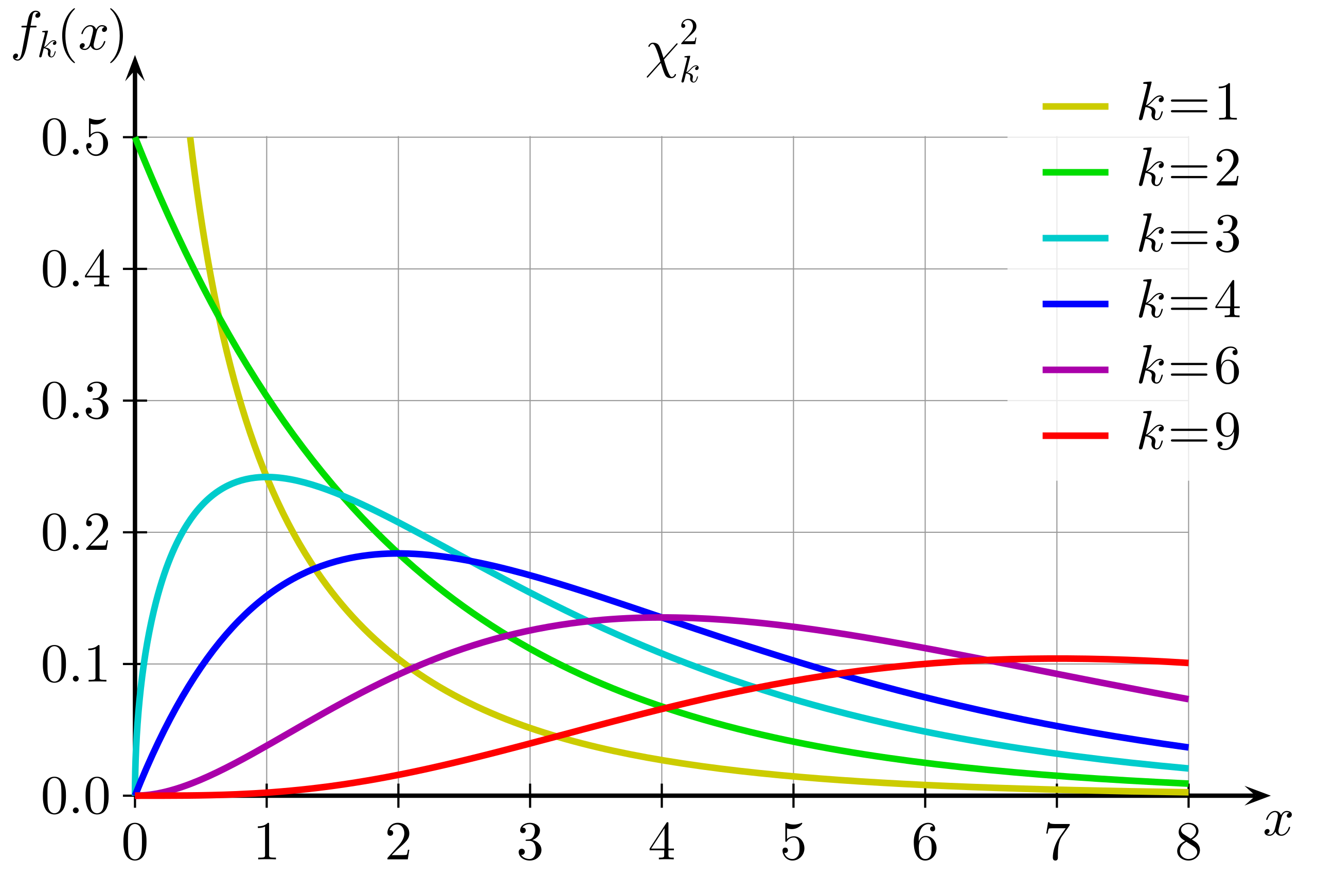
So the $p$-value for our test, which is the probability that we'd get a statistic at least as large as $6.67$ given that your theoretical frequencies are accurate, would be $$p = P(x \ge 6.67 \mid k = 2) =\int_{6.67}^\infty \frac12 e^{-\frac12 x}\, dx = e^{-\frac12 (6.67)} \approx 0.0357$$

Thus, the $\chi^2$ statistic for my sample is high enough that I can be pretty suspicious of your claim.

Theoretically speaking, the $\chi^2$ distribution with $k$ degrees of freedom is the sum of the squares of $k$ samples of the standard normal distribution $\cal N(0, 1)$. Why does the $\chi^2$ statistic follow this distribution, given that no normality was specified there? It helps to rewrite the statistic: $$\chi^2 = N\sum_{i=1}^n \frac{(e_i-t_i)^2}{t_i} = \sum_{i=1}^n \frac{N^2(e_i-t_i)^2}{Nt_i} = \sum_{i=1}^n \frac{(Ne_i-Nt_i)^2}{Nt_i}$$

Given that $N$ is the number of samples and $e_i$ and $t_i$ are the empirical and theoretical frequencies of category $i$, $Ne_i$ is simply the number of samples in category $i$, and $Nt_i$ the number of samples expected to be in category $i$. The value $Ne_i$ can be considered as the sum of $N$ samples from Bernoulli distributions with identical parameter $t_i$; each one has mean $t_i$ and variance $t_i(1-t_i)$, so by the central limit theorem we can expect the distribution of the sum of $N$ samples to approximate a normal distribution with mean $Nt_i$ and variance $Nt_i(1-t_i)$. This is where the normality in the $\chi^2$ statistic comes from, though showing that it's the sum of standard normal distributions is a bit tricky.

4. Student's t-Distribution

The statistician William Gosset, while working at a brewery, devised a test for determining whether two normal distributions with the same variance have the same mean; his employer, not wanting him to publish with his real name, had him use a pseudonym. He chose “Student”, and his test — really a family of tests all going by the same name — became known as Student's $t$-test.

Suppose we have $m$ samples $a_1, \ldots, a_m \sim \cal N(\mu_a, \sigma^2)$ and $n$ samples $b_1, \ldots, b_n \sim \cal N(\mu_b, \sigma^2)$. For instance, suppose I go around administering IQ tests — four members of the anime club get 122, 109, 116, and 128, while five members of the book club get 98, 117, 104, 110, and 108. To test the null hypothesis that the means are equal — that $\mu_a = \mu_b$ — we use the test statistic $$t = \frac{\overline a - \overline b}{\sqrt{\left(\frac1m + \frac1n\right)\left(\frac{(m-1)s_a^2 + (n-1)s_b^2}{m+n-2}\right)}} $$

Here, $s_a$ and $s_b$ are the usual estimators of the variances of each population, and it is assumed that these variances are similar to one another. (This is one of a large amount of related test statistics, see here for others). In our example, this evaluates to 2.244.

If the null hypothesis is true, the distribution of $t$ will follow the Student's $t$ distribution; like the $\chi^2$ distribution, this takes as a parameter a number of degrees of freedom $k$, generally taken to be the total number of samples minus two (subtract one for each group). The formula for $\operatorname{St}(k)$ is given by: $$P(x \mid k) = \frac{\Gamma\left(\frac{k+1}{2}\right)}{\Gamma\left(\frac{k}{2}\right)\sqrt{\pi k}} \left(1+\frac{x^2}{k}\right)^{-\frac{k+1}{2}}$$

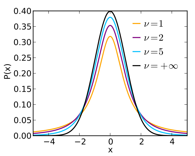
Assuming the null hypothesis that $\mu_a = \mu_b$, our statistic $t$ would be sampled from $\operatorname{St}(8)$; I'll choose to calculate our $p$-value to be the probability that the absolute value of $t$ is larger than 2.244, since a priori there's no reason to believe that a statistically significant deviation would go in any particular direction. This $p$ value is given by $$p = P(|t| \ge 2.244 \mid k = 7) = 2 \cdot P(t \ge 2.244 \mid k = 7) = 2\int_{2.244}^\infty \frac{48}{15\pi\sqrt{7}}\left(\frac{x^2+7}{7}\right)^{-4}\, dx$$ I'm not going to do this integral myself, but Wolfram|Alpha gives $p \approx 0.0597$, which, while suggestive, is not significant.

Appendix B. Results on Distributions and Priors

1. On Functional Differentiation and Lagrange Multipliers

Functional Differentiation

A functional is a map from a space of functions into the real numbers; they're generally called via brackets. For instance, the entropy functional is given by $$H[P] = -\int_X P(x)\ln P(x)\, dx$$

Just as functions can be differentiated with respect to their variables at certain numbers, functionals can be differentiated with respect to their variables at certain functions. The idea is as follows: if we take a functional $F$, an arbitrary function $\phi$, and an extremely small $\epsilon$, then $F[P+\epsilon\phi]$ should look like $F[P]$ with a small addition that depends on $\phi$. Specifically, there should be another function $f$ such that $F[P+\epsilon \phi] = F[P] + \int_X f(x) \cdot (\epsilon \phi(x))\, dx$.

The function $f$ which satisfies $\lim_{\epsilon \to 0} \frac{F[P+\epsilon \phi] - F[P]}{\epsilon} = \int f(x)\phi(x)\, dx$ is known as the functional derivative of $F$, and is generally written as $\frac{\delta F}{\delta P}$.
!tab $F$ can be said to reach a maximum at some function $q$ when there is no arbitrarily small change that can be made to $q$ which increases the value of the functional. In other words, $q$ is a maximum of $F$ when the functional derivative of $F$ is zero at $q$ no matter the choice of $\phi$.

Lagrange Multipliers

When we want to find the function $q$ that maximizes $F$ subject to some specific constraint, for instance $G[q] = k$, we may use a Lagrange multiplier. This is a functional $\lambda G$, with $\lambda \in \mathbb R$, which is added to $F$ to produce the new functional $F_\lambda = F + \lambda (G-k)$. The justification for this is as follows: the calculus of variations guarantees that any maximum of $F$ satisfying $G[q] = k$ will also maximize $F_\lambda$ for some $\lambda$. Hence, to find this $q$, we maximize $F_\lambda$, keeping $\lambda$ an arbitrary real number; $q$ will be dependent on $\lambda$, and finding that particular $\lambda$ such that $G[q]=k$ gives us our final $q$.

Laplace Approximation

Suppose we have a smooth function $f: \mathbb R^d \to \mathbb R$. The Taylor expansion of $f$ about $\vec v_0$ is given by $$f(\vec v) = f(\vec v_0) + \sum_{n=1}^\infty \frac{1}{n!} \sum_{\substack{0 \le n_1, \ldots, n_d \le n \\ \\ n_1 + \ldots + n_d = n}} \left.\frac{\partial^nf}{\partial ^{n_1}x_1 \cdots \partial^{n_d} x_d}\right|_{\vec v_0}\prod_{i=1}^d (\vec v - \vec v_0)_{i}^{n_i}$$ The first sum iterates over each order of the expansion, while the second sum iterates over all assignments of non-negative numbers to each dimension which total to the order. For instance, for the first-order $n=1$ expansion, the only possible assignments that the second sum can iterate over are those that pick out exactly one $n_i$ corresponding to one dimension. As such, the first-order Taylor expansion is $$f(\vec v) \approx f(\vec v_0) + \sum_{i=1}^d \frac{\partial f}{\partial x_i} (\vec v-\vec v_0)_i = f(\vec v_0) + (\vec v -\vec v_0)^T\nabla f(\vec v_0) $$ Hence, it simply adds to $f(\vec v_0)$ the dot product of the difference with the gradient of $f$ at $\vec v_0$. The second-order Taylor expansion further adds the sum $\sum_{i=1}^d\sum_{j=1}^d \frac{\partial^2 f}{\partial x_i\partial x_j} (\vec v-\vec v_0)_i (\vec v-\vec v_0)_j$, which can be expressed as the inner product $\frac12(\vec v - \vec v_0)^T H_f(\vec v_0) (\vec v - \vec v_0)$, where $[H_f(\vec v_0)]_{ij} = \frac{\partial^2 f}{\partial x_i \partial x_j}|_{\vec v_0}$.

We're interested in calculating the integral $\int_{} e^{nf(\vec v)}\, d\vec v$. To do this, we find the maximum $\vec v_0$ of $f$, and, to second order, Taylor expand $f$ around that maximum. Because $\vec v_0$ is a maximum, $\nabla f$ will disappear, leaving us with the known integral $$\int_{\mathbb R^n} e^{nf(\vec v)}\,d\vec v = e^{nf(\vec v_0)} \int _{\mathbb R^n} e^{\frac n2 (\vec v - \vec v_0)^TH_f(\vec v_0)(\vec v- \vec v_0)}\, d\vec v = e^{nf(\vec v)}\left(\frac{2\pi}{n}\right)^{d/2}|\det H_f(\vec v_0)|^{-\frac12}$$

Conjugate Priors

One particularly nice trick Bayesians use is the use of conjugate priors: suppose we have some data $D$ from a distribution $P(x \mid \theta)$ which is part of some family and a prior $P(\theta)$ that falls into some second family, e.g. it is a normal distribution. We say that this second family is a conjugate prior for the first family if the posterior distribution $P(\theta \mid x)$ is also part of this second family, albeit with different parameters.

I used this trick above: the conjugate prior for a normal distribution with known variance $\sigma^2$ is another normal distribution with unknown mean and variance. What this means is: if we have data $D$ sampled from some normal distribution $\cal N(\mu, \sigma^2)$, $\sigma^2$ known, and we set this conjugate prior on the parameter $\mu$, supposing $P(\mu) = \cal N(\mu_0, \sigma^2_0)$, then $P(\mu \mid D)$ will also be a normal distribution, this time with updated mean $\mu'_0 = \frac{\sigma^2\mu_0 + n\sigma_0^2\overline D}{\sigma^2 + n\sigma_0^2}$ and variance $(\sigma_0^2)' = \frac{\sigma^2\sigma_0^2}{\sigma^2+n\sigma_0^2}$. Some depth of thought is required here: we are not just dealing with the parameter $\mu$ of the distribution governing the data, but also with the parameters $\mu_0, \sigma^2_0$ of the distribution governing our beliefs about those parameters. These secondary parameters are known as hyperparameters. If we wanted, we could place priors on these hyperparameters; these would be known as hyperpriors, and their own parameters as hyperhyperparameters, but we won't go that far.

Another example: The conjugate prior for the Bernoulli distribution is the beta distribution $$P(p \mid \alpha, \beta) = \frac{\Gamma(\alpha+\beta)}{\Gamma(\alpha)\Gamma(\beta)} p^{\alpha-1} (1-p)^{\beta-1}$$ This means that if we have some data $D$ from a Bernoulli distribution $P(x\mid p) \sim \operatorname{Bern}(p)$, and a beta-distributed prior $P(p \mid \alpha, \beta) \sim \operatorname{Beta}(\alpha, \beta)$, then the posterior $P(p \mid D)$ will also be a beta distribution, with updated parameters $\alpha' = \alpha + \sum_{i=1}^n D_i$ and $\beta' = \beta + \sum_{i=1}^n (1-D_i)$; we add the number of successes to $\alpha$ and the number of failures to $\beta$ to get the posterior distribution. For instance, if we start off with $\alpha = 1, \beta = 1$, which places a uniform prior over $p$, then after observing five heads (successes) and two tails (failures), our posterior for $p$ will be $\operatorname{Beta}(6, 3)$, or $P(p = p_0 \mid \alpha = 6, \beta = 3) = 21p_0^5(1-p_0)^2$. The MAP estimate for $p$ is $5/7$, which is precisely the number of heads divided by the total number of flips.

2. The Maximum Entropy Distribution is Normal

Consider the problem of finding the distribution on $\mathbb R$ with maximum entropy among all those distributions with known mean $\mu$ and known variance $\sigma^2$. Three Lagrange multipliers come into play here, since we have to make sure that the probability distribution $P$ not only has that particular mean and that particular variance, but integrates to one as well. Hence, the functional $F$ that we want to differentiate will be given by $$F[P] = -\int P(x)\ln P(x)\, dx + \lambda_1 \int xP(x)\, dx + \lambda_2 \int (x-\mu)^2P(x)\, dx + \lambda_3 \int P(x)\, dx - \lambda_1\mu - \lambda_2 \sigma^2 - \lambda_3$$ Plugging this in to the functional derivative formula $\lim_{\epsilon \to 0} \frac{F[P+\epsilon \phi] - F[P]}{\epsilon} = \int \frac{\delta F}{\delta P}\phi(x)\, dx$, the Lagrange multiplier parts, relying only linearly on $P(x)$, simplify immediately, giving us $$\lim_{\epsilon \to 0} \frac{F[P+\epsilon \phi] - F[P]}{\epsilon} = \int (\lambda_1 x + \lambda_2 (x-\mu)^2 + \lambda_3)\phi(x)\, dx - \lim_{\epsilon \to 0} \frac{1}{\epsilon} \left[\int(P(x)+\epsilon \phi(x))\ln(P(x)+\epsilon \phi(x))\, dx - \int P(x)\ln P(x)\, dx\right]$$ The term in the limit simplifies as $$(P(x)+\epsilon\phi(x))\ln(P(x)+\epsilon \phi(x)) - P(x)\ln P(x)\\ = P(x)\left[\ln( P(x)+\epsilon\phi(x))-\ln P(x)\right] + \epsilon \phi(x) \ln(P(x)+\epsilon \phi(x))$$ $$= P(x) \left(\ln\frac{P(x)+\epsilon\phi(x)}{P(x)}\right) + \epsilon \phi(x) \left((\ln P(x)) + \frac{\epsilon \phi(x)}{P(x)} + O(\epsilon^2)\right) $$ $$= P(x)\left(\frac{\epsilon \phi(x)}{P(x)} + O(\epsilon^2)\right) + \epsilon \phi(x)\ln P(x) + O(\epsilon^2) \\ = \epsilon \phi(x) (1+ \ln P(x)) + O(\epsilon^2)$$ Dividing by $\epsilon$ and taking the limit as $\epsilon \to 0$ yields $\phi(x)(1+\ln P(x))$, allowing us to complete the functional derivative as $$\lim_{\epsilon \to 0} \frac{F[P+\epsilon \phi] - F[P]}{\epsilon} = \int \overbrace{(\lambda_1 x + \lambda_2(x-\mu)^2 + \lambda_3 -1 - \ln P(x))}^{=\delta F/\delta P}\phi(x)\, dx$$ Hence, we maximize by setting $\lambda_1 x + \lambda_2(x-\mu)^2 + \lambda_3 - 1 - \ln P(x) = 0$, or $P(x) = C\operatorname{exp}(\lambda_1 x + \lambda_2 (x-\mu)^2)$, where $C = e^{\lambda_3-1}$ is the normalization constant. Finally, we solve for the Lagrange multipliers by calculating the total probability, mean, and variance of $P(x)$: $$1 = \int C e^{\lambda_1 x + \lambda_2(x-\mu)^2}\, dx = C\frac{\sqrt{\pi} e^{\lambda_2\mu^2-(\lambda_1-2\lambda_2\mu)^2/4\lambda_2}}{\sqrt{-\lambda_2}} \implies C = \frac{\sqrt{-\lambda_2}}{\sqrt{\pi} e^{\lambda_2\mu^2-(\lambda_1-2\lambda_2\mu)^2/4\lambda_2}}$$ $$\mu = \int xCe^{\lambda_1 x + \lambda_2(x-\mu)^2}\, dx %= Ce^{\lambda_2\mu^2}\int xe^{\lambda_2x^2+(\lambda_1-2\lambda_2\mu)x}\, dx = Ce^{\lambda_2\mu^2} \frac{(\lambda_1-2\lambda_2\mu)\sqrt\pi }{-2\lambda_2\sqrt{-\lambda_2}}e^{(\lambda_1-2\lambda_2\mu)^2/(-4\lambda_2)}$$ $$= Ce^{\lambda_2\mu^2} \frac{(\lambda_1-2\lambda_2\mu) }{-2\lambda_2}e^{(\lambda_1-2\lambda_2\mu)^2/(-4\lambda_2)} = \frac{(\lambda_1-2\lambda_2\mu)}{-2\lambda_2} = -\frac12 \frac{\lambda_1}{\lambda_2} + \mu$$ $$\implies \lambda_1 = 0, \ C = \left(\int e^{\lambda_2(x-\mu)^2}\,dx\right)^{-1} = \left(\frac{\sqrt{\pi}}{\sqrt{-\lambda_2}}\right)^{-1} = \sqrt{\frac{-\lambda_2}{\pi}}$$ $$\sigma^2 = \int C (x-\mu)^2 e^{\lambda_2(x-\mu)^2}\,dx = \frac C2 \sqrt{\frac{\pi}{-\lambda_2^3}} = -\frac{1}{2\lambda_2} \implies \lambda_2 = -\frac{1}{2\sigma^2}, \ C = \frac{1}{\sqrt{2\pi\sigma^2}}$$ Plugging this back into the definition of $P$, we end up with our final answer: $$P(x) = Ce^{\lambda_2(x-\mu)^2} = \frac{1}{\sqrt{2\pi\sigma^2}} e^{-\frac{1}{2}\frac{(x-\mu)^2}{\sigma^2}} = \cal N(\mu, \sigma^2)$$

Therefore, among all those distributions with a given mean and variance, the one with maximum entropy is precisely the normal distribution with that mean and variance.

3. Maximal Data Information Prior for Normal with Known Mean

For a normal distribution with known mean $\mu$ and unknown variance $s = \sigma^2$, the entropy is $\frac12\ln(2\pi\sigma^2) + \frac12$, giving us $$G = \int P(s)\ln{\sqrt s}\, ds - \int P(s)\ln P(s)\, ds + \text{const.}$$

Add the Lagrange multiplier $\lambda \int P(s)\, ds$ to $G$ to get a new functional $G_\lambda[P]$. We calculate its functional derivative: $$\int \frac{\delta G_\lambda[P]}{\delta P}(s)\phi(s)\, ds = \lim_{\epsilon \to 0} \frac{G_\lambda[P+\epsilon\phi] - G_\lambda[P]}{\epsilon}$$ $$ \lim_{\epsilon \to 0} \frac{1}{\epsilon}\left[\int (P(s)+\epsilon \phi(s))\ln\sqrt s\, ds - \int (P(s)+\epsilon \phi(s))\ln (P(s)+\epsilon \phi(s))\, ds \right.\\ + \left.\lambda \int (P(s)+\epsilon\phi(s))\, ds - \int P(s)\ln{\sqrt s}\, ds + \int P(s)\ln P(s) \, ds - \lambda \int P(s)\, ds\right]$$ $$ = \lim_{\epsilon \to 0} \frac{1}{\epsilon}\left[\int \epsilon\phi(s)\ln \sqrt{s}\, ds +\int P(s) \ln \frac{P(s)}{P(s)+\epsilon \phi(s)}\, ds \right. \\ - \int \epsilon \phi(s)\ln(P(s)+\epsilon \phi(s))\, ds + \lambda \int \epsilon \phi(s)\,ds\left. \right] $$ $$= \int \phi(s)(\lambda + \ln\sqrt{s}) \, ds + \lim_{\epsilon \to 0} \left[\int \frac1\epsilon P(s) \left(\frac{-\epsilon \phi(s)}{P(s)} - O(\epsilon^2)\right)\, ds - \int \phi(s)\ln(P(s)+\epsilon \phi(s))\, ds \right] $$ $$ = \int \phi(s)(\lambda - 1 + \ln \sqrt{s} + \ln P(s))\, ds$$ which implies that $\frac{\delta G_\lambda[P]}{\delta P} = \lambda + 1 + \ln \sqrt{s} + \ln P(s)$; we set $\lambda + 1 + \ln \sqrt{s} + \ln P(s) = 0$ to get $P(s) = e^{-\lambda-1-\ln \sqrt{s}} = Cs^{-\frac12} = C\sigma^{-1}$, where $C = e^{-\lambda-1}$ is the normalization constant. Unfortunately, this prior, which is the same as the Jeffreys prior, is non-normalizable: $\int_0^\infty s^{-\frac12}\, ds = \left[2\sqrt{s}\right]_0^\infty = \infty$.

4. Empirical Bayes for the Poisson Distribution With Gamma Prior

Given data $D = \{k_1, \ldots, k_n\}\sim \operatorname{Pois}(\lambda)$ and a prior $\lambda \sim \operatorname{Gamma}(\alpha, \beta)$, we want to find the $\alpha, \beta$ that maximize $P(D \mid \alpha, \beta)$. Recall that for $k$ a single data point, these distributions are given by $$P(k \mid \lambda) = \frac{\lambda^ke^{-\lambda}}{k!} \qquad P(\lambda \mid \alpha, \beta) = \frac{\beta^{\alpha}\lambda^{\alpha-1}e^{-\beta\lambda}}{\Gamma(\alpha)}$$ The first step is to write out $P(D \mid \alpha, \beta)$: $$P(D \mid \alpha, \beta) = \int_{0}^\infty P(D \mid \lambda)P(\lambda \mid \alpha, \beta)\, d\lambda \\ = \int_{0}^\infty \left(\prod_{i=1}^n\frac{\lambda^{k_i}e^{-\lambda}}{{k_i}!}\right)\frac{\beta^\alpha \lambda^{\alpha-1}e^{-\beta\lambda}}{\Gamma(\alpha)}\, d\lambda = \frac{\beta^\alpha}{\Gamma(\alpha)F}\int_0^{\infty}\lambda^{S+\alpha-1}e^{-(n+\beta)\lambda}\, d\lambda$$ where $S = \sum_{i=1}^n k_i$ and $F = \prod_{i=1}^n k_i!$.

In general, the integral $\int_0^\infty x^ae^{-bx}\,dx$ evaluates to $\Gamma(a+1)/b^{a+1}$ (easily derived from the definition of the gamma function), so the above integral evaluates to $$\frac{\beta^\alpha}{\Gamma(\alpha)F} \frac{\Gamma(\alpha+S)}{(\beta+n)^{\alpha+S}} = \frac 1F \frac{\beta^\alpha}{(\beta+n)^{\alpha+S}}\frac{\Gamma(\alpha+S)}{\Gamma(\alpha)}$$ This is what we want to maximize w.r.t. $\alpha$ and $\beta$. We'll take the logarithm and then take the partial derivatives: letting $\ell = \ln P(D \mid \alpha, \beta)$, we have $$\ell = \alpha \ln \beta - (\alpha+S)\ln(\beta + n) + \ln \Gamma(\alpha + S) - \ln \Gamma(\alpha) - \ln F \\ \frac{\partial \ell}{\partial \alpha} = \ln \beta - \ln(\beta + n) + \psi(\alpha+S) - \psi(\alpha)\\ \frac{\partial \ell}{\partial \beta} = \frac{\alpha}{\beta} - \frac{\alpha+S}{\beta+n} $$ $$= \frac{\alpha\beta + \alpha n -\alpha \beta - \beta S}{\beta(n+\beta)} = \frac{\alpha n - \beta S}{\beta(n+\beta)}$$ Here, $\psi(x) = \frac{d}{dx} \ln \Gamma(x)$ is the digamma function, putting us squarely in Special Function Hell. To maximize, we need to set the derivatives equal to zero, solve for $\alpha, \beta$, and then make sure we haven't hit a saddle point by checking that $\ell_{\alpha\alpha}\ell_{\beta\beta} > \ell_{\alpha\beta}^2$ and either one of $\ell_{\alpha\alpha},\ell_{\beta\beta}$ is negative.

It is clear that $\partial \ell/\partial \beta = 0$ when $\alpha n = \beta S$, or $\alpha/\beta = S/n = \overline D$.

Solving for $\partial \ell/\partial \alpha = 0$ is extremely hard; one terrible approach is to use the identity $\Gamma(\alpha+S)/\Gamma(\alpha) \approx \alpha^S$, leading us to the line of reasoning $$\ell \approx \alpha \ln \beta - (\alpha + S) \ln (\beta + n) + S \ln \alpha - \ln F \\ \frac{\partial \ell}{\partial \alpha} \approx \ln \beta - \ln (\beta + n) + \frac{S}{\alpha} = 0 \implies \frac S\alpha = \ln(\beta + n) - \ln \beta = \ln\left(1 + \frac\beta n\right)$$ $$\implies 1+\frac\beta n = e^{S/\alpha} \implies \beta = n(e^{S/\alpha}-1) = ne^{n/\beta}-n \\ \implies n/\beta+1 = (n/\beta)e^{n/\beta}$$ The equation $x +1 = xe^x$ has precisely one positive solution at $x \approx 0.806$, so we must have $\beta \approx n/0.806 \approx 1.24n$, and correspondingly $\alpha = \beta S/n \approx 1.24S$.

This is a really bad approximation and just seems morally wrong, so I won't accept it. However, we should at least check that this is a maximum: we have $$\ell_{\alpha\alpha} \approx \psi_1(\alpha+S)-\psi_1(\alpha), \ell_{\beta\beta} = \frac{-S\beta(n+\beta) - (n+2\beta)}{\beta^2(n+\beta)^2}, \ell_{\alpha\beta} = \ell_{\beta\alpha} = 0$$

Here, $\psi_1$ is the trigamma function; it is strictly decreasing, so $\ell_{\alpha\alpha}$ is always negative. $\ell_{\beta\beta}$ is clearly always negative as well, so we are at a maximum. In fact, the fact that both of these are always negative implies that there is a unique global maximum, and therefore a unique maximum likelihood estimate of $\alpha, \beta$.

Work: To solve for $\partial \ell/\partial \alpha = 0$, we may make use of the following identity: for a positive integer $n$, $\psi(x+n)-\psi(x) = \sum_{i=0}^{n-1}\frac{1}{x+i}$. Each data point, being the number of times something happened in a given period of time, is a positive integer, making their sum $S$ a positive integer as well. Hence, we have $$\frac{\partial \ell}{\partial \alpha} = \ln \beta - \ln(\beta + n) + \sum_{i=0}^{S-1} \frac{1}{\alpha+i}$$ I've tried a lot of approaches, but I can't find a way to set this equal to zero that isn't either intractable or equivalent to $\alpha/\beta = S/n$. Oh well. The sum is rather difficult to work with, so we'll approximate it by the integral $\int_0^S \frac{1}{\alpha+x}\, dx = \ln (\alpha + S)-\ln\alpha$, giving us $$\frac{\partial \ell}{\partial \alpha} = \ln \frac{\beta}{\beta+n} + \ln \frac{\alpha+S}{\alpha} = \ln \frac{\beta (\alpha+S)}{(\beta+n)\alpha} = 0 \\ \implies \frac{\beta(\alpha+S)}{(\beta+n)\alpha} = 1 \implies \beta \alpha + \beta S = \beta \alpha + n\alpha \\ \implies \beta S = n\alpha \implies \frac{\alpha}{\beta} = \frac{S}{n} = \overline D$$ We get the exact same result. Since the approximation becomes arbitrarily accurate in the limit, We apply the Euler-Maclaurin formula to “simplify” the sum: $$\sum_{i=a}^{b-1} f(i) \approx \int_a^b f(x)\, dx + \frac{f(a)-f(b)}{2} + \sum_{i=1}^\infty \frac{B_{2i}}{(2i)!}\left(f^{(2i-1)}(b)-f^{(2i-1)}(a)\right) \\ {\small \sum_{i=0}^{S-1} \frac{1}{\alpha+i} \approx \ln \frac{S+\alpha}{\alpha} + \frac{\frac1\alpha-\frac{1}{S+\alpha}}{2} + \sum_{i=1}^\infty \frac{B_{2i}}{(2i)!}(-1)^{2i-1}(2i-1)!\left[(S+\alpha)^{-2i}-\alpha^{-2i}\right]}$$ $$ = \ln\left(\frac{S+\alpha}{\alpha}\right) + \frac{S}{2\alpha(S+\alpha)} - \sum_{i=1}^\infty \frac{B_{2i}}{2i}\left[(S+\alpha)^{-2i}-\alpha^{-2i}\right]$$ Applying $\alpha = \beta S/n$, we get $$0= \ln \left(\frac{\beta}{\beta+n} \right)+ \ln\left(\frac{n+\beta }{\beta }\right) + \frac{n^2}{2S\beta (n+\beta)} - \sum_{i=1}^\infty \frac{B_{2i}}{2i}\left(\frac nS\right)^{2i}\left[(n+\beta)^{-2i}-\beta^{-2i}\right]$$ The first two terms cancel out, so if we simply ignore the sum, we get leaving us with $$\frac{1}{\beta(n+\beta)} = \frac{2S}{n^2}\sum_{i=1}^\infty \frac{B_{2i}}{2i}\left(\frac nS\right)^{2i}\frac{\beta^{2i}-(n+\beta)^{2i}}{\beta^{2i}(n+\beta)^{2i}} \\ \implies 1 = \sum_{i=1}^\infty \frac{B_{2i}}{ni}\left(\frac{n}{S\beta(n+\beta)}\right)^{2i-1}(\beta^{2i}-(n+\beta)^{2i})$$ The first two terms of this sum are $$1 = -\frac{1}{6n}\left(\frac{n}{S\beta(n+\beta)}\right)((n+\beta)^2-\beta^2) +\frac{1}{30n}\frac{n^3}{S^3\beta^3(n+\beta)^3}((n+\beta)^2+\beta^2)((n+\beta)^2-\beta^2)$$ $$ \implies 30\frac{S^3}{n^2} +10\frac{S^2}{n^2} = \frac{1}{\beta^3} +\frac{n}{\beta^2}+ \frac{1}{(n+\beta)^2} -\frac{n}{(n+\beta)^3} - 5\frac{S^2}{n^2} \frac{n}{\beta} + 5\frac{S^2}{n^2} \frac{n}{(n+\beta)}$$ For large $n$, this will reduce to $$10\frac{S^2}{n^2}(3S+1) = \frac{n}{\beta^2} $$

5. MAP for the Mean of a Gaussian Distribution with Known Variance

Take a normal distribution with known variance $\sigma^2$ and unknown mean $\mu$, from which data $D = \{x_1, \ldots, x_n\}$ is sampled. Placing a normal prior ${\cal N}(\mu_0, \sigma_0^2)$, the MAP estimate for $\mu$ is given by $${\small \widehat \mu = \operatorname{argmax}_\mu \frac{P(D \mid \mu)P(\mu)}{P(D)} = \operatorname{argmax}_\mu\frac{1}{P(D)} \frac{1}{\sqrt{2\pi\sigma_0^2}}e^{-\frac12\frac{(\mu-\mu_0)^2}{\sigma_0^2}} \prod_{i=1}^n \frac{1}{\sqrt{2\pi\sigma^2}}e^{-\frac12\frac{(x_i-\mu)^2}{\sigma^2}}}$$ Since we're just maximizing with respect to $\mu$, we can not only remove all constants which do not depend on $\mu$ (including the difficult integral $P(D)$), but apply any order-preserving function we want without affecting the maximization process. Removing these constants, and applying the logarithmic function, we simplify this as $${\small \widehat \mu = \operatorname{argmax}_\mu -\frac12\frac{(\mu-\mu_0)^2}{\sigma_0^2} - \frac{1}{2\sigma^2} \sum_{i=1}^n (x_i-\mu)^2 = \operatorname{argmin}_\mu \sigma^2(\mu-\mu_0)^2 + \sigma_0^2\sum_{i=1}^n (x_i-\mu)^2 } \\ {\small = \operatorname{argmin}_\mu \sigma^2\mu^2-2\sigma^2\mu_0\mu + \sigma_0^2\sum_{i=1}^n \mu^2-2\mu{x_i} = \operatorname{argmin}_\mu (\sigma^2+n\sigma_0^2)\mu^2 - 2\left(\sigma^2\mu_0+n\sigma_0^2\overline D\right)\mu}$$ The usual way to minimize such a function is to take the derivative with respect to $\mu$ and set it equal to zero. Doing this gives us $$2(\sigma^2+n\sigma^2_0)\mu - 2(\sigma^2\mu_0 + n\sigma_0^2\overline D) = 0 \\ \,\\\implies \widehat \mu(D) = \frac{\sigma^2\mu_0+n\sigma_0^2\overline D}{\sigma^2+n\sigma_0^2} = \frac{\left(\frac{\sigma^2}{\sigma_0^2}\right)\mu_0 + n\overline D}{\left(\frac{\sigma^2}{\sigma_0^2}\right) + n}$$

This is a weighted estimate of the prior and sample means, which weighs the sample mean more heavily insofar as it based off of a greater number of samples and weighs the prior mean more heavily insofar as its variance is lower than that of the known population variance — beautifully intuitive. In the case where $D = \{x\}$ is a single number and $\sigma^2=\sigma_0^2$, the MAP estimator $\widehat \mu(D)$ will be perfectly in between $\mu_0$ and $x$.

6. The MSE Bayes Estimator is the Posterior Mean

Endnotes